
In a earlier publish, we confirmed how you can use tfprobability – the R interface to TensorFlow Likelihood – to construct a multilevel, or partial pooling mannequin of tadpole survival in otherwise sized (and thus, differing in inhabitant quantity) tanks.
A totally pooled mannequin would have resulted in a world estimate of survival rely, regardless of tank, whereas an unpooled mannequin would have realized to foretell survival rely for every tank individually. The previous method doesn’t keep in mind totally different circumstances; the latter doesn’t make use of widespread data. (Additionally, it clearly has no predictive use until we need to make predictions for the exact same entities we used to coach the mannequin.)
In distinction, a partially pooled mannequin allows you to make predictions for the acquainted, in addition to new entities: Simply use the suitable prior.
Assuming we are actually concerned about the identical entities – why would we need to apply partial pooling?
For a similar causes a lot effort in machine studying goes into devising regularization mechanisms. We don’t need to overfit an excessive amount of to precise measurements, be they associated to the identical entity or a category of entities. If I need to predict my coronary heart charge as I get up subsequent morning, primarily based on a single measurement I’m taking now (let’s say it’s night and I’m frantically typing a weblog publish), I higher keep in mind some info about coronary heart charge conduct generally (as an alternative of simply projecting into the long run the precise worth measured proper now).
Within the tadpole instance, this implies we count on generalization to work higher for tanks with many inhabitants, in comparison with extra solitary environments. For the latter ones, we higher take a peek at survival charges from different tanks, to complement the sparse, idiosyncratic data accessible.
Or utilizing the technical time period, within the latter case we hope for the mannequin to shrink its estimates towards the general imply extra noticeably than within the former.
Any such data sharing is already very helpful, however it will get higher. The tadpole mannequin is a various intercepts mannequin, as McElreath calls it (or random intercepts, as it’s typically – confusingly – known as ) – intercepts referring to the way in which we make predictions for entities (right here: tanks), with no predictor variables current. So if we are able to pool details about intercepts, why not pool details about slopes as effectively? This may permit us to, as well as, make use of relationships between variables learnt on totally different entities within the coaching set.
In order you might need guessed by now, various slopes (or random slopes, if you’ll) is the subject of as we speak’s publish. Once more, we take up an instance from McElreath’s e-book, and present how you can accomplish the identical factor with tfprobability.
Espresso, please
Not like the tadpole case, this time we work with simulated information. That is the info McElreath makes use of to introduce the various slopes modeling approach; he then goes on and applies it to one of many e-book’s most featured datasets, the pro-social (or detached, quite!) chimpanzees. For as we speak, we stick with the simulated information for 2 causes: First, the subject material per se is non-trivial sufficient; and second, we need to hold cautious observe of what our mannequin does, and whether or not its output is sufficiently near the outcomes McElreath obtained from Stan .
So, the situation is that this. Cafés differ in how common they’re. In a preferred café, if you order espresso, you’re more likely to wait. In a much less common café, you’ll probably be served a lot quicker. That’s one factor.
Second, all cafés are typically extra crowded within the mornings than within the afternoons. Thus within the morning, you’ll wait longer than within the afternoon – this goes for the favored in addition to the much less common cafés.
By way of intercepts and slopes, we are able to image the morning waits as intercepts, and the resultant afternoon waits as arising as a result of slopes of the strains becoming a member of every morning and afternoon wait, respectively.
So after we partially-pool intercepts, we now have one “intercept prior” (itself constrained by a previous, in fact), and a set of café-specific intercepts that may differ round it. Once we partially-pool slopes, we now have a “slope prior” reflecting the general relationship between morning and afternoon waits, and a set of café-specific slopes reflecting the person relationships. Cognitively, that implies that when you’ve got by no means been to the Café Gerbeaud in Budapest however have been to cafés earlier than, you might need a less-than-uninformed concept about how lengthy you’ll wait; it additionally implies that for those who usually get your espresso in your favourite nook café within the mornings, and now you move by there within the afternoon, you’ve got an approximate concept how lengthy it’s going to take (specifically, fewer minutes than within the mornings).
So is that every one? Really, no. In our situation, intercepts and slopes are associated. If, at a much less common café, I all the time get my espresso earlier than two minutes have handed, there may be little room for enchancment. At a extremely common café although, if it may simply take ten minutes within the mornings, then there may be fairly some potential for lower in ready time within the afternoon. So in my prediction for this afternoon’s ready time, I ought to issue on this interplay impact.
So, now that we now have an concept of what that is all about, let’s see how we are able to mannequin these results with tfprobability. However first, we really should generate the info.
Simulate the info
We instantly comply with McElreath in the way in which the info are generated.
##### Inputs wanted to generate the covariance matrix between intercepts and slopes #####

# common morning wait time
a <- 3.5
# common distinction afternoon wait time
# we wait much less within the afternoons
b <- -1
# normal deviation within the (café-specific) intercepts
sigma_a <- 1
# normal deviation within the (café-specific) slopes
sigma_b <- 0.5
# correlation between intercepts and slopes
# the upper the intercept, the extra the wait goes down
rho <- -0.7


##### Generate the covariance matrix #####

# technique of intercepts and slopes
mu <- c(a, b)
# normal deviations of means and slopes
sigmas <- c(sigma_a, sigma_b)
# correlation matrix
# a correlation matrix has ones on the diagonal and the correlation within the off-diagonals
rho <- matrix(c(1, rho, rho, 1), nrow = 2)
# now matrix multiply to get covariance matrix
cov_matrix <- diag(sigmas) %*% rho %*% diag(sigmas)


##### Generate the café-specific intercepts and slopes #####

# 20 cafés general
n_cafes <- 20

library(MASS)
set.seed(5) # used to copy instance
# multivariate distribution of intercepts and slopes
vary_effects <- mvrnorm(n_cafes , mu ,cov_matrix)
# intercepts are within the first column
a_cafe <- vary_effects[ ,1]
# slopes are within the second
b_cafe <- vary_effects[ ,2]


##### Generate the precise wait occasions #####

set.seed(22)
# 10 visits per café
n_visits <- 10

# alternate values for mornings and afternoons within the information body
afternoon <- rep(0:1, n_visits * n_cafes/2)
# information for every café are consecutive rows within the information body
cafe_id <- rep(1:n_cafes, every = n_visits)

# the regression equation for the imply ready time
mu <- a_cafe[cafe_id] + b_cafe[cafe_id] * afternoon
# normal deviation of ready time inside cafés
sigma <- 0.5 # std dev inside cafes
# generate situations of ready occasions
wait <- rnorm(n_visits * n_cafes, mu, sigma)

d <- information.body(cafe = cafe_id, afternoon = afternoon, wait = wait)
Take a glimpse on the information:
Observations: 200
Variables: 3
$ cafe      <int> 1, 1, 1, 1, 1, 1, 1, 1, 1, 1, 2, 2, 2, 2, 2, 2, 2, 2, 2, 2, 3,...
$ afternoon <int> 0, 1, 0, 1, 0, 1, 0, 1, 0, 1, 0, 1, 0, 1, 0, 1, 0, 1, 0, 1, 0,...
$ wait      <dbl> 3.9678929, 3.8571978, 4.7278755, 2.7610133, 4.1194827, 3.54365,...
On to constructing the mannequin.
The mannequin
As within the earlier publish on multi-level modeling, we use tfd_joint_distribution_sequential to outline the mannequin and Hamiltonian Monte Carlo for sampling. Contemplate having a look on the first part of that publish for a fast reminder of the general process.
Earlier than we code the mannequin, let’s shortly get library loading out of the way in which. Importantly, once more similar to within the earlier publish, we have to set up a grasp construct of TensorFlow Likelihood, as we’re making use of very new options not but accessible within the present launch model. The identical goes for the R packages tensorflow and tfprobability: Please set up the respective growth variations from github.
Now right here is the mannequin definition. We’ll undergo it step-by-step immediately.
mannequin <- perform(cafe_id) {
  tfd_joint_distribution_sequential(
      checklist(
        # rho, the prior for the correlation matrix between intercepts and slopes
        tfd_cholesky_lkj(2, 2),
        # sigma, prior variance for the ready time
        tfd_sample_distribution(tfd_exponential(charge = 1), sample_shape = 1),
        # sigma_cafe, prior of variances for intercepts and slopes (vector of two)
        tfd_sample_distribution(tfd_exponential(charge = 1), sample_shape = 2),
        # b, the prior imply for the slopes
        tfd_sample_distribution(tfd_normal(loc = -1, scale = 0.5), sample_shape = 1),
        # a, the prior imply for the intercepts
        tfd_sample_distribution(tfd_normal(loc = 5, scale = 2), sample_shape = 1),
        # mvn, multivariate distribution of intercepts and slopes
        # form: batch dimension, 20, 2
        perform(a,b,sigma_cafe,sigma,chol_rho)
          tfd_sample_distribution(
            tfd_multivariate_normal_tri_l(
              loc = tf$concat(checklist(a,b), axis = -1L),
              scale_tril = tf$linalg$LinearOperatorDiag(sigma_cafe)$matmul(chol_rho)),
            sample_shape = n_cafes),
        # ready time
        # form ought to be batch dimension, 200
        perform(mvn, a, b, sigma_cafe, sigma)
          tfd_independent(
            # want to tug out the proper cafe_id within the center column
            tfd_normal(
              loc = (tf$collect(mvn[ , , 1], cafe_id, axis = -1L) +
                       tf$collect(mvn[ , , 2], cafe_id, axis = -1L) * afternoon),
              scale=sigma),  # Form [batch,  1]
        reinterpreted_batch_ndims=1
        )
    )
  )
}
The primary 5 distributions are priors. First, we now have the prior for the correlation matrix.
Mainly, this may be an LKJ distribution of form 2x2 and with focus parameter equal to 2.
For efficiency causes, we work with a model that inputs and outputs Cholesky elements as an alternative:
# rho, the prior correlation matrix between intercepts and slopes
tfd_cholesky_lkj(2, 2)
What sort of prior is that this? As McElreath retains reminding us, nothing is extra instructive than sampling from the prior. For us to see what’s happening, we use the bottom LKJ distribution, not the Cholesky one:
corr_prior <- tfd_lkj(2, 2)
correlation <- (corr_prior %>% tfd_sample(100))[ , 1, 2] %>% as.numeric()
library(ggplot2)
information.body(correlation) %>% ggplot(aes(x = correlation)) + geom_density()
So this prior is reasonably skeptical about robust correlations, however fairly open to studying from information.
The following distribution in line
# sigma, prior variance for the ready time
tfd_sample_distribution(tfd_exponential(charge = 1), sample_shape = 1)
is the prior for the variance of the ready time, the final distribution within the checklist.
Subsequent is the prior distribution of variances for the intercepts and slopes. This prior is similar for each circumstances, however we specify a sample_shape of two to get two particular person samples.
# sigma_cafe, prior of variances for intercepts and slopes (vector of two)
tfd_sample_distribution(tfd_exponential(charge = 1), sample_shape = 2)
Now that we now have the respective prior variances, we transfer on to the prior means. Each are regular distributions.
# b, the prior imply for the slopes
tfd_sample_distribution(tfd_normal(loc = -1, scale = 0.5), sample_shape = 1)
# a, the prior imply for the intercepts
tfd_sample_distribution(tfd_normal(loc = 5, scale = 2), sample_shape = 1)On to the guts of the mannequin, the place the partial pooling occurs. We’re going to assemble partially-pooled intercepts and slopes for the entire cafés. Like we stated above, intercepts and slopes usually are not impartial; they work together. Thus, we have to use a multivariate regular distribution.
The means are given by the prior means outlined proper above, whereas the covariance matrix is constructed from the above prior variances and the prior correlation matrix.
The output form right here is set by the variety of cafés: We would like an intercept and a slope for each café.
# mvn, multivariate distribution of intercepts and slopes
# form: batch dimension, 20, 2
perform(a,b,sigma_cafe,sigma,chol_rho)
  tfd_sample_distribution(
    tfd_multivariate_normal_tri_l(
      loc = tf$concat(checklist(a,b), axis = -1L),
      scale_tril = tf$linalg$LinearOperatorDiag(sigma_cafe)$matmul(chol_rho)),
  sample_shape = n_cafes)
Lastly, we pattern the precise ready occasions.
This code pulls out the proper intercepts and slopes from the multivariate regular and outputs the imply ready time, depending on what café we’re in and whether or not it’s morning or afternoon.
        # ready time
        # form: batch dimension, 200
        perform(mvn, a, b, sigma_cafe, sigma)
          tfd_independent(
            # want to tug out the proper cafe_id within the center column
            tfd_normal(
              loc = (tf$collect(mvn[ , , 1], cafe_id, axis = -1L) +
                       tf$collect(mvn[ , , 2], cafe_id, axis = -1L) * afternoon),
              scale=sigma),
        reinterpreted_batch_ndims=1
        )
Earlier than operating the sampling, it’s all the time a good suggestion to do a fast verify on the mannequin.
n_cafes <- 20
cafe_id <- tf$forged((d$cafe - 1) %% 20, tf$int64)

afternoon <- d$afternoon
wait <- d$wait
We pattern from the mannequin after which, verify the log likelihood.
m <- mannequin(cafe_id)

s <- m %>% tfd_sample(3)
m %>% tfd_log_prob(s)
We would like a scalar log likelihood per member within the batch, which is what we get.
tf.Tensor([-466.1392 -149.92587 -196.51688], form=(3,), dtype=float32)Working the chains
The precise Monte Carlo sampling works similar to within the earlier publish, with one exception. Sampling occurs in unconstrained parameter house, however on the finish we have to get legitimate correlation matrix parameters rho and legitimate variances sigma and sigma_cafe. Conversion between areas is finished by way of TFP bijectors. Fortunately, this isn’t one thing we now have to do as customers; all we have to specify are applicable bijectors. For the conventional distributions within the mannequin, there may be nothing to do.
constraining_bijectors <- checklist(
  # be sure that the rho[1:4] parameters are legitimate for a Cholesky issue
  tfb_correlation_cholesky(),
  # be sure that variance is optimistic
  tfb_exp(),
  # be sure that variance is optimistic
  tfb_exp(),
  tfb_identity(),
  tfb_identity(),
  tfb_identity()
)
Now we are able to arrange the Hamiltonian Monte Carlo sampler.
n_steps <- 500
n_burnin <- 500
n_chains <- 4

# arrange the optimization goal
logprob <- perform(rho, sigma, sigma_cafe, b, a, mvn)
  m %>% tfd_log_prob(checklist(rho, sigma, sigma_cafe, b, a, mvn, wait))

# preliminary states for the sampling process
c(initial_rho, initial_sigma, initial_sigma_cafe, initial_b, initial_a, initial_mvn, .) %<-%
  (m %>% tfd_sample(n_chains))

# HMC sampler, with the above bijectors and step dimension adaptation
hmc <- mcmc_hamiltonian_monte_carlo(
  target_log_prob_fn = logprob,
  num_leapfrog_steps = 3,
  step_size = checklist(0.1, 0.1, 0.1, 0.1, 0.1, 0.1)
) %>%
  mcmc_transformed_transition_kernel(bijector = constraining_bijectors) %>%
  mcmc_simple_step_size_adaptation(target_accept_prob = 0.8,
                                   num_adaptation_steps = n_burnin)
Once more, we are able to acquire extra diagnostics (right here: step sizes and acceptance charges) by registering a hint perform:
trace_fn <- perform(state, pkr) {
  checklist(pkr$inner_results$inner_results$is_accepted,
       pkr$inner_results$inner_results$accepted_results$step_size)
}
Right here, then, is the sampling perform. Notice how we use tf_function to place it on the graph. No less than as of as we speak, this makes an enormous distinction in sampling efficiency when utilizing keen execution.
run_mcmc <- perform(kernel) {
  kernel %>% mcmc_sample_chain(
    num_results = n_steps,
    num_burnin_steps = n_burnin,
    current_state = checklist(initial_rho,
                         tf$ones_like(initial_sigma),
                         tf$ones_like(initial_sigma_cafe),
                         initial_b,
                         initial_a,
                         initial_mvn),
    trace_fn = trace_fn
  )
}

run_mcmc <- tf_function(run_mcmc)
res <- hmc %>% run_mcmc()

mcmc_trace <- res$all_states
So how do our samples look, and what will we get by way of posteriors? Let’s see.
Outcomes
At this second, mcmc_trace is an inventory of tensors of various shapes, depending on how we outlined the parameters. We have to do a little bit of post-processing to have the ability to summarise and show the outcomes.
# the precise mcmc samples
# for the hint plots, we need to have them in form (500, 4, 49)
# that's: (variety of steps, variety of chains, variety of parameters)
samples <- abind(
  # rho 1:4
  as.array(mcmc_trace[[1]] %>% tf$reshape(checklist(tf$forged(n_steps, tf$int32), tf$forged(n_chains, tf$int32), 4L))),
  # sigma
  as.array(mcmc_trace[[2]]),
  # sigma_cafe 1:2
  as.array(mcmc_trace[[3]][ , , 1]),
  as.array(mcmc_trace[[3]][ , , 2]),
  # b
  as.array(mcmc_trace[[4]]),
  # a
  as.array(mcmc_trace[[5]]),
  # mvn 10:49
  as.array( mcmc_trace[[6]] %>% tf$reshape(checklist(tf$forged(n_steps, tf$int32), tf$forged(n_chains, tf$int32), 40L))),
  alongside = 3)

# the efficient pattern sizes
# we wish them in form (4, 49), which is (variety of chains * variety of parameters)
ess <- mcmc_effective_sample_size(mcmc_trace)
ess <- cbind(
  # rho 1:4
  as.matrix(ess[[1]] %>% tf$reshape(checklist(tf$forged(n_chains, tf$int32), 4L))),
  # sigma
  as.matrix(ess[[2]]),
  # sigma_cafe 1:2
  as.matrix(ess[[3]][ , 1, drop = FALSE]),
  as.matrix(ess[[3]][ , 2, drop = FALSE]),
  # b
  as.matrix(ess[[4]]),
  # a
  as.matrix(ess[[5]]),
  # mvn 10:49
  as.matrix(ess[[6]] %>% tf$reshape(checklist(tf$forged(n_chains, tf$int32), 40L)))
  )

# the rhat values
# we wish them in form (49), which is (variety of parameters)
rhat <- mcmc_potential_scale_reduction(mcmc_trace)
rhat <- c(
  # rho 1:4
  as.double(rhat[[1]] %>% tf$reshape(checklist(4L))),
  # sigma
  as.double(rhat[[2]]),
  # sigma_cafe 1:2
  as.double(rhat[[3]][1]),
  as.double(rhat[[3]][2]),
  # b
  as.double(rhat[[4]]),
  # a
  as.double(rhat[[5]]),
  # mvn 10:49
  as.double(rhat[[6]] %>% tf$reshape(checklist(40L)))
  )
Hint plots
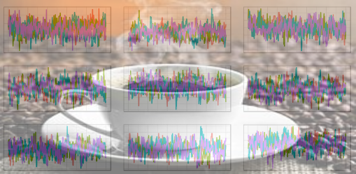
How effectively do the chains combine?
prep_tibble <- perform(samples) {
  as_tibble(samples, .name_repair = ~ c("chain_1", "chain_2", "chain_3", "chain_4")) %>%
    add_column(pattern = 1:n_steps) %>%
    collect(key = "chain", worth = "worth", -pattern)
}

plot_trace <- perform(samples) {
  prep_tibble(samples) %>%
    ggplot(aes(x = pattern, y = worth, colour = chain)) +
    geom_line() +
    theme_light() +
    theme(legend.place = "none",
          axis.title = element_blank(),
          axis.textual content = element_blank(),
          axis.ticks = element_blank())
}

plot_traces <- perform(sample_array, num_params) {
  plots <- purrr::map(1:num_params, ~ plot_trace(sample_array[ , , .x]))
  do.name(grid.organize, plots)
}

plot_traces(samples, 49)
Superior! (The primary two parameters of rho, the Cholesky issue of the correlation matrix, want to remain fastened at 1 and 0, respectively.)
Now, on to some abstract statistics on the posteriors of the parameters.
Parameters
Like final time, we show posterior means and normal deviations, in addition to the very best posterior density interval (HPDI). We add efficient pattern sizes and rhat values.
column_names <- c(
  paste0("rho_", 1:4),
  "sigma",
  paste0("sigma_cafe_", 1:2),
  "b",
  "a",
  c(rbind(paste0("a_cafe_", 1:20), paste0("b_cafe_", 1:20)))
)

all_samples <- matrix(samples, nrow = n_steps * n_chains, ncol = 49)
all_samples <- all_samples %>%
  as_tibble(.name_repair = ~ column_names)

all_samples %>% glimpse()

means <- all_samples %>%
  summarise_all(checklist (imply)) %>%
  collect(key = "key", worth = "imply")

sds <- all_samples %>%
  summarise_all(checklist (sd)) %>%
  collect(key = "key", worth = "sd")

hpdis <-
  all_samples %>%
  summarise_all(checklist(~ checklist(hdi(.) %>% t() %>% as_tibble()))) %>%
   unnest()

 hpdis_lower <- hpdis %>% choose(-accommodates("higher")) %>%
   rename(lower0 = decrease) %>%
   collect(key = "key", worth = "decrease") %>%
   organize(as.integer(str_sub(key, 6))) %>%
   mutate(key = column_names)

 hpdis_upper <- hpdis %>% choose(-accommodates("decrease")) %>%
   rename(upper0 = higher) %>%
   collect(key = "key", worth = "higher") %>%
   organize(as.integer(str_sub(key, 6))) %>%
   mutate(key = column_names)

abstract <- means %>%
  inner_join(sds, by = "key") %>%
  inner_join(hpdis_lower, by = "key") %>%
  inner_join(hpdis_upper, by = "key")

ess <- apply(ess, 2, imply)

summary_with_diag <- abstract %>% add_column(ess = ess, rhat = rhat)
print(summary_with_diag, n = 49)
# A tibble: 49 x 7
key imply sd decrease higher ess rhat
<chr> <dbl> <dbl> <dbl> <dbl> <dbl> <dbl>
1 rho_1 1 0 1 1 NaN NaN
2 rho_2 0 0 0 0 NaN NaN
3 rho_3 -0.517 0.176 -0.831 -0.195 42.4 1.01
4 rho_4 0.832 0.103 0.644 1.000 46.5 1.02
5 sigma 0.473 0.0264 0.420 0.523 424. 1.00
6 sigma_cafe_1 0.967 0.163 0.694 1.29 97.9 1.00
7 sigma_cafe_2 0.607 0.129 0.386 0.861 42.3 1.03
8 b -1.14 0.141 -1.43 -0.864 95.1 1.00
9 a 3.66 0.218 3.22 4.07 75.3 1.01
10 a_cafe_1 4.20 0.192 3.83 4.57 83.9 1.01
11 b_cafe_1 -1.13 0.251 -1.63 -0.664 63.6 1.02
12 a_cafe_2 2.17 0.195 1.79 2.54 59.3 1.01
13 b_cafe_2 -0.923 0.260 -1.42 -0.388 46.0 1.01
14 a_cafe_3 4.40 0.195 4.02 4.79 56.7 1.01
15 b_cafe_3 -1.97 0.258 -2.52 -1.51 43.9 1.01
16 a_cafe_4 3.22 0.199 2.80 3.57 58.7 1.02
17 b_cafe_4 -1.20 0.254 -1.70 -0.713 36.3 1.01
18 a_cafe_5 1.86 0.197 1.45 2.20 52.8 1.03
19 b_cafe_5 -0.113 0.263 -0.615 0.390 34.6 1.04
20 a_cafe_6 4.26 0.210 3.87 4.67 43.4 1.02
21 b_cafe_6 -1.30 0.277 -1.80 -0.713 41.4 1.05
22 a_cafe_7 3.61 0.198 3.23 3.98 44.9 1.01
23 b_cafe_7 -1.02 0.263 -1.51 -0.489 37.7 1.03
24 a_cafe_8 3.95 0.189 3.59 4.31 73.1 1.01
25 b_cafe_8 -1.64 0.248 -2.10 -1.13 60.7 1.02
26 a_cafe_9 3.98 0.212 3.57 4.37 76.3 1.03
27 b_cafe_9 -1.29 0.273 -1.83 -0.776 57.8 1.05
28 a_cafe_10 3.60 0.187 3.24 3.96 104. 1.01
29 b_cafe_10 -1.00 0.245 -1.47 -0.512 70.4 1.00
30 a_cafe_11 1.95 0.200 1.56 2.35 55.9 1.03
31 b_cafe_11 -0.449 0.266 -1.00 0.0619 42.5 1.04
32 a_cafe_12 3.84 0.195 3.46 4.22 76.0 1.02
33 b_cafe_12 -1.17 0.259 -1.65 -0.670 62.5 1.03
34 a_cafe_13 3.88 0.201 3.50 4.29 62.2 1.02
35 b_cafe_13 -1.81 0.270 -2.30 -1.29 48.3 1.03
36 a_cafe_14 3.19 0.212 2.82 3.61 65.9 1.07
37 b_cafe_14 -0.961 0.278 -1.49 -0.401 49.9 1.06
38 a_cafe_15 4.46 0.212 4.08 4.91 62.0 1.09
39 b_cafe_15 -2.20 0.290 -2.72 -1.59 47.8 1.11
40 a_cafe_16 3.41 0.193 3.02 3.78 62.7 1.02
41 b_cafe_16 -1.07 0.253 -1.54 -0.567 48.5 1.05
42 a_cafe_17 4.22 0.201 3.82 4.60 58.7 1.01
43 b_cafe_17 -1.24 0.273 -1.74 -0.703 43.8 1.01
44 a_cafe_18 5.77 0.210 5.34 6.18 66.0 1.02
45 b_cafe_18 -1.05 0.284 -1.61 -0.511 49.8 1.02
46 a_cafe_19 3.23 0.203 2.88 3.65 52.7 1.02
47 b_cafe_19 -0.232 0.276 -0.808 0.243 45.2 1.01
48 a_cafe_20 3.74 0.212 3.35 4.21 48.2 1.04
49 b_cafe_20 -1.09 0.281 -1.58 -0.506 36.5 1.05So what do we now have? In the event you run this “stay”, for the rows a_cafe_n resp. b_cafe_n, you see a pleasant alternation of white and purple coloring: For all cafés, the inferred slopes are damaging.
The inferred slope prior (b) is round -1.14, which isn’t too far off from the worth we used for sampling: 1.
The rho posterior estimates, admittedly, are much less helpful until you’re accustomed to compose Cholesky elements in your head. We compute the ensuing posterior correlations and their imply:
-0.5166775The worth we used for sampling was -0.7, so we see the regularization impact. In case you’re questioning, for a similar information Stan yields an estimate of -0.5.
Lastly, let’s show equivalents to McElreath’s figures illustrating shrinkage on the parameter (café-specific intercepts and slopes) in addition to the end result (morning resp. afternoon ready occasions) scales.
Shrinkage
As anticipated, we see that the person intercepts and slopes are pulled in direction of the imply – the extra, the additional away they’re from the middle.
# similar to McElreath, compute unpooled estimates instantly from information
a_empirical <- d %>%
  filter(afternoon == 0) %>%
  group_by(cafe) %>%
  summarise(a = imply(wait)) %>%
  choose(a)

b_empirical <- d %>%
  filter(afternoon == 1) %>%
  group_by(cafe) %>%
  summarise(b = imply(wait)) %>%
  choose(b) -
  a_empirical

empirical_estimates <- bind_cols(
  a_empirical,
  b_empirical,
  sort = rep("information", 20))

posterior_estimates <- tibble(
  a = means %>% filter(
  str_detect(key, "^a_cafe")) %>% choose(imply) %>% pull(),
  b = means %>% filter(
    str_detect(key, "^b_cafe")) %>% choose(imply)  %>% pull(),
  sort = rep("posterior", 20))

all_estimates <- bind_rows(empirical_estimates, posterior_estimates)

# compute posterior imply bivariate Gaussian
# once more following McElreath
mu_est <- c(means[means$key == "a", 2], means[means$key == "b", 2]) %>% unlist()
rho_est <- mean_rho
sa_est <- means[means$key == "sigma_cafe_1", 2] %>% unlist()
sb_est <- means[means$key == "sigma_cafe_2", 2] %>% unlist()
cov_ab <- sa_est * sb_est * rho_est
sigma_est <- matrix(c(sa_est^2, cov_ab, cov_ab, sb_est^2), ncol=2)

alpha_levels <- c(0.1, 0.3, 0.5, 0.8, 0.99)
names(alpha_levels) <- alpha_levels

contour_data <- plyr::ldply(
  alpha_levels,
  ellipse,
  x = sigma_est,
  scale = c(1, 1),
  centre = mu_est
)

ggplot() +
  geom_point(information = all_estimates, mapping = aes(x = a, y = b, colour = sort)) +
  geom_path(information = contour_data, mapping = aes(x = x, y = y, group = .id))
The identical conduct is seen on the end result scale.
wait_times  <- all_estimates %>%
  mutate(morning = a, afternoon = a + b)

# simulate from posterior means
v <- MASS::mvrnorm(1e4 , mu_est , sigma_est)
v[ ,2] <- v[ ,1] + v[ ,2] # calculate afternoon wait
# assemble empirical covariance matrix
sigma_est2 <- cov(v)
mu_est2 <- mu_est
mu_est2[2] <- mu_est[1] + mu_est[2]

contour_data <- plyr::ldply(
  alpha_levels,
  ellipse,
  x = sigma_est2 %>% unname(),
  scale = c(1, 1),
  centre = mu_est2
)

ggplot() +
  geom_point(information = wait_times, mapping = aes(x = morning, y = afternoon, colour = sort)) +
  geom_path(information = contour_data, mapping = aes(x = x, y = y, group = .id))
Wrapping up
By now, we hope we now have satisfied you of the facility inherent in Bayesian modeling, in addition to conveyed some concepts on how that is achievable with TensorFlow Likelihood. As with each DSL although, it takes time to proceed from understanding labored examples to design your individual fashions. And never simply time – it helps to have seen loads of totally different fashions, specializing in totally different duties and purposes.
On this weblog, we plan to loosely comply with up on Bayesian modeling with TFP, selecting up a number of the duties and challenges elaborated on within the later chapters of McElreath’s e-book. Thanks for studying!
