Understanding LoRA with a minimal instance

LoRA (Low-Rank Adaptation) is a brand new method for fantastic tuning giant scale pre-trained
fashions. Such fashions are often skilled on basic area information, in order to have
the utmost quantity of knowledge. With a view to get hold of higher ends in duties like chatting
or query answering, these fashions might be additional ‘fine-tuned’ or tailored on area
particular information.

It’s attainable to fine-tune a mannequin simply by initializing the mannequin with the pre-trained
weights and additional coaching on the area particular information. With the rising dimension of
pre-trained fashions, a full ahead and backward cycle requires a considerable amount of computing
sources. High quality tuning by merely persevering with coaching additionally requires a full copy of all
parameters for every activity/area that the mannequin is tailored to.

LoRA: Low-Rank Adaptation of Giant Language Fashions
proposes an answer for each issues by utilizing a low rank matrix decomposition.
It will probably cut back the variety of trainable weights by 10,000 occasions and GPU reminiscence necessities
by 3 occasions.

Methodology

The issue of fine-tuning a neural community might be expressed by discovering a (Delta Theta)
that minimizes (L(X, y; Theta_0 + DeltaTheta)) the place (L) is a loss operate, (X) and (y)
are the information and (Theta_0) the weights from a pre-trained mannequin.

We study the parameters (Delta Theta) with dimension (|Delta Theta|)
equals to (|Theta_0|). When (|Theta_0|) could be very giant, similar to in giant scale
pre-trained fashions, discovering (Delta Theta) turns into computationally difficult.
Additionally, for every activity it’s essential study a brand new (Delta Theta) parameter set, making
it much more difficult to deploy fine-tuned fashions when you’ve got greater than a
few particular duties.

LoRA proposes utilizing an approximation (Delta Phi approx Delta Theta) with (|Delta Phi| << |Delta Theta|).
The remark is that neural nets have many dense layers performing matrix multiplication,
and whereas they usually have full-rank throughout pre-training, when adapting to a selected activity
the burden updates can have a low “intrinsic dimension”.

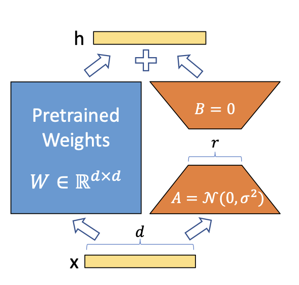
A easy matrix decomposition is utilized for every weight matrix replace (Delta theta in Delta Theta).
Contemplating (Delta theta_i in mathbb{R}^{d occasions okay}) the replace for the (i)th weight
within the community, LoRA approximates it with:

[Delta theta_i approx Delta phi_i = BA]
the place (B in mathbb{R}^{d occasions r}), (A in mathbb{R}^{r occasions d}) and the rank (r << min(d, okay)).
Thus as an alternative of studying (d occasions okay) parameters we now must study ((d + okay) occasions r) which is definitely
quite a bit smaller given the multiplicative side. In follow, (Delta theta_i) is scaled
by (frac{alpha}{r}) earlier than being added to (theta_i), which might be interpreted as a
‘studying charge’ for the LoRA replace.

LoRA doesn’t improve inference latency, as as soon as fantastic tuning is finished, you possibly can merely
replace the weights in (Theta) by including their respective (Delta theta approx Delta phi).
It additionally makes it less complicated to deploy a number of activity particular fashions on prime of 1 giant mannequin,
as (|Delta Phi|) is way smaller than (|Delta Theta|).

Implementing in torch

Now that we’ve got an concept of how LoRA works, let’s implement it utilizing torch for a
minimal downside. Our plan is the next:

1. Simulate coaching information utilizing a easy (y = X theta) mannequin. (theta in mathbb{R}^{1001, 1000}).
2. Practice a full rank linear mannequin to estimate (theta) – this might be our ‘pre-trained’ mannequin.
3. Simulate a unique distribution by making use of a change in (theta).
4. Practice a low rank mannequin utilizing the pre=skilled weights.

Let’s begin by simulating the coaching information:

library(torch)

n <- 10000
d_in <- 1001
d_out <- 1000

thetas <- torch_randn(d_in, d_out)

X <- torch_randn(n, d_in)
y <- torch_matmul(X, thetas)

We now outline our base mannequin:

mannequin <- nn_linear(d_in, d_out, bias = FALSE)

We additionally outline a operate for coaching a mannequin, which we’re additionally reusing later.
The operate does the usual traning loop in torch utilizing the Adam optimizer.
The mannequin weights are up to date in-place.

prepare <- operate(mannequin, X, y, batch_size = 128, epochs = 100) {
  choose <- optim_adam(mannequin$parameters)

  for (epoch in 1:epochs) {
    for(i in seq_len(n/batch_size)) {
      idx <- pattern.int(n, dimension = batch_size)
      loss <- nnf_mse_loss(mannequin(X[idx,]), y[idx])
      
      with_no_grad({
        choose$zero_grad()
        loss$backward()
        choose$step()  
      })
    }
    
    if (epoch %% 10 == 0) {
      with_no_grad({
        loss <- nnf_mse_loss(mannequin(X), y)
      })
      cat("[", epoch, "] Loss:", loss$merchandise(), "n")
    }
  }
}

The mannequin is then skilled:

prepare(mannequin, X, y)
#> [ 10 ] Loss: 577.075 
#> [ 20 ] Loss: 312.2 
#> [ 30 ] Loss: 155.055 
#> [ 40 ] Loss: 68.49202 
#> [ 50 ] Loss: 25.68243 
#> [ 60 ] Loss: 7.620944 
#> [ 70 ] Loss: 1.607114 
#> [ 80 ] Loss: 0.2077137 
#> [ 90 ] Loss: 0.01392935 
#> [ 100 ] Loss: 0.0004785107

OK, so now we’ve got our pre-trained base mannequin. Let’s suppose that we’ve got information from
a slighly totally different distribution that we simulate utilizing:

thetas2 <- thetas + 1

X2 <- torch_randn(n, d_in)
y2 <- torch_matmul(X2, thetas2)

If we apply out base mannequin to this distribution, we don’t get a great efficiency:

nnf_mse_loss(mannequin(X2), y2)
#> torch_tensor
#> 992.673
#> [ CPUFloatType{} ][ grad_fn = <MseLossBackward0> ]

We now fine-tune our preliminary mannequin. The distribution of the brand new information is simply slighly
totally different from the preliminary one. It’s only a rotation of the information factors, by including 1
to all thetas. Because of this the burden updates should not anticipated to be complicated, and
we shouldn’t want a full-rank replace to be able to get good outcomes.

Let’s outline a brand new torch module that implements the LoRA logic:

lora_nn_linear <- nn_module(
  initialize = operate(linear, r = 16, alpha = 1) {
    self$linear <- linear
    
    # parameters from the unique linear module are 'freezed', so they aren't
    # tracked by autograd. They're thought-about simply constants.
    purrr::stroll(self$linear$parameters, (x) x$requires_grad_(FALSE))
    
    # the low rank parameters that might be skilled
    self$A <- nn_parameter(torch_randn(linear$in_features, r))
    self$B <- nn_parameter(torch_zeros(r, linear$out_feature))
    
    # the scaling fixed
    self$scaling <- alpha / r
  },
  ahead = operate(x) {
    # the modified ahead, that simply provides the outcome from the bottom mannequin
    # and ABx.
    self$linear(x) + torch_matmul(x, torch_matmul(self$A, self$B)*self$scaling)
  }
)

We now initialize the LoRA mannequin. We are going to use (r = 1), that means that A and B might be simply
vectors. The bottom mannequin has 1001×1000 trainable parameters. The LoRA mannequin that we’re
are going to fantastic tune has simply (1001 + 1000) which makes it 1/500 of the bottom mannequin
parameters.

lora <- lora_nn_linear(mannequin, r = 1)

Now let’s prepare the lora mannequin on the brand new distribution:

prepare(lora, X2, Y2)
#> [ 10 ] Loss: 798.6073 
#> [ 20 ] Loss: 485.8804 
#> [ 30 ] Loss: 257.3518 
#> [ 40 ] Loss: 118.4895 
#> [ 50 ] Loss: 46.34769 
#> [ 60 ] Loss: 14.46207 
#> [ 70 ] Loss: 3.185689 
#> [ 80 ] Loss: 0.4264134 
#> [ 90 ] Loss: 0.02732975 
#> [ 100 ] Loss: 0.001300132 

If we take a look at (Delta theta) we’ll see a matrix stuffed with 1s, the precise transformation
that we utilized to the weights:

delta_theta <- torch_matmul(lora$A, lora$B)*lora$scaling
delta_theta[1:5, 1:5]
#> torch_tensor
#>  1.0002  1.0001  1.0001  1.0001  1.0001
#>  1.0011  1.0010  1.0011  1.0011  1.0011
#>  0.9999  0.9999  0.9999  0.9999  0.9999
#>  1.0015  1.0014  1.0014  1.0014  1.0014
#>  1.0008  1.0008  1.0008  1.0008  1.0008
#> [ CPUFloatType{5,5} ][ grad_fn = <SliceBackward0> ]

To keep away from the extra inference latency of the separate computation of the deltas,
we might modify the unique mannequin by including the estimated deltas to its parameters.
We use the add_ methodology to change the burden in-place.

with_no_grad({
  mannequin$weight$add_(delta_theta$t())  
})

Now, making use of the bottom mannequin to information from the brand new distribution yields good efficiency,
so we are able to say the mannequin is tailored for the brand new activity.

nnf_mse_loss(mannequin(X2), y2)
#> torch_tensor
#> 0.00130013
#> [ CPUFloatType{} ]

Concluding

Now that we discovered how LoRA works for this straightforward instance we are able to suppose the way it might
work on giant pre-trained fashions.

Seems that Transformers fashions are largely intelligent group of those matrix
multiplications, and making use of LoRA solely to those layers is sufficient for lowering the
fantastic tuning value by a big quantity whereas nonetheless getting good efficiency. You may see
the experiments within the LoRA paper.

After all, the concept of LoRA is easy sufficient that it may be utilized not solely to
linear layers. You may apply it to convolutions, embedding layers and really every other layer.

Picture by Hu et al on the LoRA paper