
About half a 12 months in the past, this weblog featured a publish, written by Daniel Falbel, on the right way to use Keras to categorise items of spoken language. The article received lots of consideration and never surprisingly, questions arose the right way to apply that code to totally different datasets. We’ll take this as a motivation to discover in additional depth the preprocessing accomplished in that publish: If we all know why the enter to the community seems to be the way in which it seems to be, we will modify the mannequin specification appropriately if want be.
In case you will have a background in speech recognition, and even basic sign processing, for you the introductory a part of this publish will in all probability not include a lot information. Nevertheless, you would possibly nonetheless have an interest within the code half, which exhibits the right way to do issues like creating spectrograms with present variations of TensorFlow.
Should you don’t have that background, we’re inviting you on a (hopefully) fascinating journey, barely bearing on one of many larger mysteries of this universe.
We’ll use the identical dataset as Daniel did in his publish, that’s, model 1 of the Google speech instructions dataset(Warden 2018)
The dataset consists of ~ 65,000 WAV recordsdata, of size one second or much less. Every file is a recording of one in every of thirty phrases, uttered by totally different audio system.
The purpose then is to coach a community to discriminate between spoken phrases. How ought to the enter to the community look? The WAV recordsdata include amplitudes of sound waves over time. Listed here are just a few examples, comparable to the phrases fowl, down, sheila, and visible:

A sound wave is a sign extending in time, analogously to how what enters our visible system extends in house.
At every cut-off date, the present sign depends on its previous. The apparent structure to make use of in modeling it thus appears to be a recurrent neural community.
Nevertheless, the data contained within the sound wave might be represented in an alternate manner: particularly, utilizing the frequencies that make up the sign.
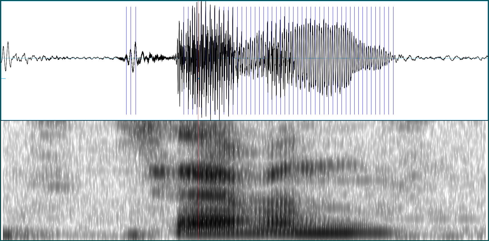
Right here we see a sound wave (prime) and its frequency illustration (backside).

Within the time illustration (known as the time area), the sign consists of consecutive amplitudes over time. Within the frequency area, it’s represented as magnitudes of various frequencies. It could seem as one of many biggest mysteries on this world which you could convert between these two with out lack of data, that’s: Each representations are primarily equal!
Conversion from the time area to the frequency area is completed utilizing the Fourier remodel; to transform again, the Inverse Fourier Remodel is used. There exist various kinds of Fourier transforms relying on whether or not time is seen as steady or discrete, and whether or not the sign itself is steady or discrete. Within the “actual world,” the place normally for us, actual means digital as we’re working with digitized alerts, the time area in addition to the sign are represented as discrete and so, the Discrete Fourier Remodel (DFT) is used. The DFT itself is computed utilizing the FFT (Quick Fourier Remodel) algorithm, leading to important speedup over a naive implementation.
Trying again on the above instance sound wave, it’s a compound of 4 sine waves, of frequencies 8Hz, 16Hz, 32Hz, and 64Hz, whose amplitudes are added and displayed over time. The compound wave right here is assumed to increase infinitely in time. In contrast to speech, which adjustments over time, it may be characterised by a single enumeration of the magnitudes of the frequencies it’s composed of. So right here the spectrogram, the characterization of a sign by magnitudes of constituent frequencies various over time, seems to be primarily one-dimensional.
Nevertheless, after we ask Praat to create a spectrogram of one in every of our instance sounds (a seven), it may appear to be this:

Right here we see a two-dimensional picture of frequency magnitudes over time (increased magnitudes indicated by darker coloring). This two-dimensional illustration could also be fed to a community, rather than the one-dimensional amplitudes. Accordingly, if we determine to take action we’ll use a convnet as a substitute of an RNN.
Spectrograms will look totally different relying on how we create them. We’ll check out the important choices in a minute. First although, let’s see what we can’t all the time do: ask for all frequencies that have been contained within the analog sign.
Above, we stated that each representations, time area and frequency area, have been primarily equal. In our digital actual world, that is solely true if the sign we’re working with has been digitized accurately, or as that is generally phrased, if it has been “correctly sampled.”
Take speech for instance: As an analog sign, speech per se is steady in time; for us to have the ability to work with it on a pc, it must be transformed to occur in discrete time. This conversion of the unbiased variable (time in our case, house in e.g. picture processing) from steady to discrete is known as sampling.
On this strategy of discretization, an important determination to be made is the sampling fee to make use of. The sampling fee must be not less than double the very best frequency within the sign. If it’s not, lack of data will happen. The best way that is most frequently put is the opposite manner spherical: To protect all data, the analog sign could not include frequencies above one-half the sampling fee. This frequency – half the sampling fee – is known as the Nyquist fee.
If the sampling fee is simply too low, aliasing takes place: Larger frequencies alias themselves as decrease frequencies. Which means that not solely can’t we get them, in addition they corrupt the magnitudes of corresponding decrease frequencies they’re being added to.
Right here’s a schematic instance of how a high-frequency sign may alias itself as being lower-frequency. Think about the high-frequency wave being sampled at integer factors (gray circles) solely:

Within the case of the speech instructions dataset, all sound waves have been sampled at 16 kHz. Which means that after we ask Praat for a spectogram, we should always not ask for frequencies increased than 8kHz. Here’s what occurs if we ask for frequencies as much as 16kHz as a substitute – we simply don’t get them:

Now let’s see what choices we do have when creating spectrograms.
Within the above easy sine wave instance, the sign stayed fixed over time. Nevertheless in speech utterances, the magnitudes of constituent frequencies change over time. Ideally thus, we’d have a precise frequency illustration for each cut-off date. As an approximation to this perfect, the sign is split into overlapping home windows, and the Fourier remodel is computed for every time slice individually. That is known as the Brief Time Fourier Remodel (STFT).
Once we compute the spectrogram by way of the STFT, we have to inform it what measurement home windows to make use of, and the way massive to make the overlap. The longer the home windows we use, the higher the decision we get within the frequency area. Nevertheless, what we acquire in decision there, we lose within the time area, as we’ll have fewer home windows representing the sign. It is a basic precept in sign processing: Decision within the time and frequency domains are inversely associated.
To make this extra concrete, let’s once more have a look at a easy instance. Right here is the spectrogram of an artificial sine wave, composed of two parts at 1000 Hz and 1200 Hz. The window size was left at its (Praat) default, 5 milliseconds:

We see that with a brief window like that, the 2 totally different frequencies are mangled into one within the spectrogram.
Now enlarge the window to 30 milliseconds, and they’re clearly differentiated:

The above spectrogram of the phrase “seven” was produced utilizing Praats default of 5 milliseconds. What occurs if we use 30 milliseconds as a substitute?

We get higher frequency decision, however on the value of decrease decision within the time area. The window size used throughout preprocessing is a parameter we would need to experiment with later, when coaching a community.
One other enter to the STFT to play with is the kind of window used to weight the samples in a time slice. Right here once more are three spectrograms of the above recording of seven, utilizing, respectively, a Hamming, a Hann, and a Gaussian window:

Whereas the spectrograms utilizing the Hann and Gaussian home windows don’t look a lot totally different, the Hamming window appears to have launched some artifacts.
Preprocessing choices don’t finish with the spectrogram. A preferred transformation utilized to the spectrogram is conversion to mel scale, a scale based mostly on how people really understand variations in pitch. We don’t elaborate additional on this right here, however we do briefly touch upon the respective TensorFlow code under, in case you’d prefer to experiment with this.
Previously, coefficients remodeled to Mel scale have generally been additional processed to acquire the so-called Mel-Frequency Cepstral Coefficients (MFCCs). Once more, we simply present the code. For glorious studying on Mel scale conversion and MFCCs (together with the explanation why MFCCs are much less typically used these days) see this publish by Haytham Fayek.
Again to our unique process of speech classification. Now that we’ve gained a little bit of perception in what’s concerned, let’s see the right way to carry out these transformations in TensorFlow.
Code shall be represented in snippets in line with the performance it gives, so we could immediately map it to what was defined conceptually above.
A whole instance is on the market right here. The entire instance builds on Daniel’s unique code as a lot as attainable, with two exceptions:
-
The code runs in keen in addition to in static graph mode. Should you determine you solely ever want keen mode, there are just a few locations that may be simplified. That is partly associated to the truth that in keen mode, TensorFlow operations rather than tensors return values, which we will immediately cross on to TensorFlow capabilities anticipating values, not tensors. As well as, much less conversion code is required when manipulating intermediate values in R.
-
With TensorFlow 1.13 being launched any day, and preparations for TF 2.0 operating at full velocity, we would like the code to necessitate as few modifications as attainable to run on the subsequent main model of TF. One massive distinction is that there’ll now not be a
contribmodule. Within the unique publish,contribwas used to learn within the.wavrecordsdata in addition to compute the spectrograms. Right here, we are going to use performance fromtf.audioandtf.signas a substitute.
All operations proven under will run inside tf.dataset code, which on the R facet is achieved utilizing the tfdatasets bundle.
To clarify the person operations, we have a look at a single file, however later we’ll additionally show the info generator as a complete.
For stepping by way of particular person strains, it’s all the time useful to have keen mode enabled, independently of whether or not in the end we’ll execute in keen or graph mode:
We choose a random .wav file and decode it utilizing tf$audio$decode_wav.This may give us entry to 2 tensors: the samples themselves, and the sampling fee.
fname <- "knowledge/speech_commands_v0.01/fowl/00b01445_nohash_0.wav"
wav <- tf$audio$decode_wav(tf$read_file(fname))
wav$sample_rate accommodates the sampling fee. As anticipated, it’s 16000, or 16kHz:
sampling_rate <- wav$sample_rate %>% as.numeric()
sampling_rate16000The samples themselves are accessible as wav$audio, however their form is (16000, 1), so now we have to transpose the tensor to get the standard (batch_size, variety of samples) format we want for additional processing.
samples <- wav$audio
samples <- samples %>% tf$transpose(perm = c(1L, 0L))
samples
tf.Tensor(
[[-0.00750732 0.04653931 0.02041626 ... -0.01004028 -0.01300049
-0.00250244]], form=(1, 16000), dtype=float32)Computing the spectogram
To compute the spectrogram, we use tf$sign$stft (the place stft stands for Brief Time Fourier Remodel). stft expects three non-default arguments: Moreover the enter sign itself, there are the window measurement, frame_length, and the stride to make use of when figuring out the overlapping home windows, frame_step. Each are expressed in items of variety of samples. So if we determine on a window size of 30 milliseconds and a stride of 10 milliseconds …
window_size_ms <- 30
window_stride_ms <- 10
… we arrive on the following name:
samples_per_window <- sampling_rate * window_size_ms/1000
stride_samples <-  sampling_rate * window_stride_ms/1000

stft_out <- tf$sign$stft(
  samples,
  frame_length = as.integer(samples_per_window),
  frame_step = as.integer(stride_samples)
)
Inspecting the tensor we received again, stft_out, we see, for our single enter wave, a matrix of 98 x 257 advanced values:
tf.Tensor(
[[[ 1.03279948e-04+0.00000000e+00j -1.95371482e-04-6.41121820e-04j
   -1.60833192e-03+4.97534114e-04j ... -3.61620914e-05-1.07343149e-04j
   -2.82576875e-05-5.88812982e-05j  2.66879797e-05+0.00000000e+00j]
   ...
   ]],
form=(1, 98, 257), dtype=complex64)
Right here 98 is the variety of intervals, which we will compute upfront, based mostly on the variety of samples in a window and the dimensions of the stride:
257 is the variety of frequencies we obtained magnitudes for. By default, stft will apply a Quick Fourier Remodel of measurement smallest energy of two larger or equal to the variety of samples in a window, after which return the fft_length / 2 + 1 distinctive parts of the FFT: the zero-frequency time period and the positive-frequency phrases.
In our case, the variety of samples in a window is 480. The closest enclosing energy of two being 512, we find yourself with 512/2 + 1 = 257 coefficients.
This too we will compute upfront:
Again to the output of the STFT. Taking the elementwise magnitude of the advanced values, we get hold of an power spectrogram:
magnitude_spectrograms <- tf$abs(stft_out)If we cease preprocessing right here, we are going to normally need to log remodel the values to raised match the sensitivity of the human auditory system:
log_magnitude_spectrograms = tf$log(magnitude_spectrograms + 1e-6)Mel spectrograms and Mel-Frequency Cepstral Coefficients (MFCCs)
If as a substitute we select to make use of Mel spectrograms, we will get hold of a change matrix that can convert the unique spectrograms to Mel scale:
lower_edge_hertz <- 0
upper_edge_hertz <- 2595 * log10(1 + (sampling_rate/2)/700)
num_mel_bins <- 64L
num_spectrogram_bins <- magnitude_spectrograms$form[-1]$worth

linear_to_mel_weight_matrix <- tf$sign$linear_to_mel_weight_matrix(
  num_mel_bins,
  num_spectrogram_bins,
  sampling_rate,
  lower_edge_hertz,
  upper_edge_hertz
)
Making use of that matrix, we get hold of a tensor of measurement (batch_size, variety of intervals, variety of Mel coefficients) which once more, we will log-compress if we would like:
mel_spectrograms <- tf$tensordot(magnitude_spectrograms, linear_to_mel_weight_matrix, 1L)
log_mel_spectrograms <- tf$log(mel_spectrograms + 1e-6)
Only for completeness’ sake, lastly we present the TensorFlow code used to additional compute MFCCs. We don’t embody this within the full instance as with MFCCs, we would wish a unique community structure.
num_mfccs <- 13
mfccs <- tf$sign$mfccs_from_log_mel_spectrograms(log_mel_spectrograms)[, , 1:num_mfccs]
Accommodating different-length inputs
In our full instance, we decide the sampling fee from the primary file learn, thus assuming all recordings have been sampled on the similar fee. We do enable for various lengths although. For instance in our dataset, had we used this file, simply 0.65 seconds lengthy, for demonstration functions:
fname <- "knowledge/speech_commands_v0.01/fowl/1746d7b6_nohash_0.wav"we’d have ended up with simply 63 intervals within the spectrogram. As now we have to outline a hard and fast input_size for the primary conv layer, we have to pad the corresponding dimension to the utmost attainable size, which is n_periods computed above.
The padding really takes place as a part of dataset definition. Let’s shortly see dataset definition as a complete, leaving out the attainable technology of Mel spectrograms.
data_generator <- operate(df,
                           window_size_ms,
                           window_stride_ms) {

  # assume sampling fee is identical in all samples
  sampling_rate <-
    tf$audio$decode_wav(tf$read_file(tf$reshape(df$fname[[1]], checklist()))) %>% .$sample_rate

  samples_per_window <- (sampling_rate * window_size_ms) %/% 1000L
  stride_samples <-  (sampling_rate * window_stride_ms) %/% 1000L

  n_periods <-
    tf$form(
      tf$vary(
        samples_per_window %/% 2L,
        16000L - samples_per_window %/% 2L,
        stride_samples
      )
    )[1] + 1L

  n_fft_coefs <-
    (2 ^ tf$ceil(tf$log(
      tf$forged(samples_per_window, tf$float32)
    ) / tf$log(2)) /
      2 + 1L) %>% tf$forged(tf$int32)

  ds <- tensor_slices_dataset(df) %>%
    dataset_shuffle(buffer_size = buffer_size)

  ds <- ds %>%
    dataset_map(operate(obs) {
      wav <-
        tf$audio$decode_wav(tf$read_file(tf$reshape(obs$fname, checklist())))
      samples <- wav$audio
      samples <- samples %>% tf$transpose(perm = c(1L, 0L))

      stft_out <- tf$sign$stft(samples,
                                 frame_length = samples_per_window,
                                 frame_step = stride_samples)

      magnitude_spectrograms <- tf$abs(stft_out)
      log_magnitude_spectrograms <- tf$log(magnitude_spectrograms + 1e-6)

      response <- tf$one_hot(obs$class_id, 30L)

      enter <- tf$transpose(log_magnitude_spectrograms, perm = c(1L, 2L, 0L))
      checklist(enter, response)
    })

  ds <- ds %>%
    dataset_repeat()

  ds %>%
    dataset_padded_batch(
      batch_size = batch_size,
      padded_shapes = checklist(tf$stack(checklist(
        n_periods, n_fft_coefs,-1L
      )),
      tf$fixed(-1L, form = form(1L))),
      drop_remainder = TRUE
    )
}
The logic is identical as described above, solely the code has been generalized to work in keen in addition to graph mode. The padding is taken care of by dataset_padded_batch(), which must be advised the utmost variety of intervals and the utmost variety of coefficients.
Time for experimentation
Constructing on the full instance, now’s the time for experimentation: How do totally different window sizes have an effect on classification accuracy? Does transformation to the mel scale yield improved outcomes? You may also need to strive passing a non-default window_fn to stft (the default being the Hann window) and see how that impacts the outcomes. And naturally, the easy definition of the community leaves lots of room for enchancment.
Talking of the community: Now that we’ve gained extra perception into what’s contained in a spectrogram, we would begin asking, is a convnet actually an enough answer right here? Usually we use convnets on pictures: two-dimensional knowledge the place each dimensions signify the identical form of data. Thus with pictures, it’s pure to have sq. filter kernels.
In a spectrogram although, the time axis and the frequency axis signify basically various kinds of data, and it’s not clear in any respect that we should always deal with them equally. Additionally, whereas in pictures, the interpretation invariance of convnets is a desired characteristic, this isn’t the case for the frequency axis in a spectrogram.
Closing the circle, we uncover that as a consequence of deeper data concerning the topic area, we’re in a greater place to cause about (hopefully) profitable community architectures. We depart it to the creativity of our readers to proceed the search…
