Posit AI Weblog: Picture segmentation with U-Internet

Positive, it’s good when I’ve an image of some object, and a neural community can inform me what sort of object that’s. Extra realistically, there could be a number of salient objects in that image, and it tells me what they’re, and the place they’re. The latter job (generally known as object detection) appears particularly prototypical of up to date AI purposes that on the similar time are intellectually fascinating and ethically questionable. It’s completely different with the topic of this put up: Profitable picture segmentation has a variety of undeniably helpful purposes. For instance, it’s a sine qua non in drugs, neuroscience, biology and different life sciences.

So what, technically, is picture segmentation, and the way can we prepare a neural community to do it?

Picture segmentation in a nutshell

Say we’ve got a picture with a bunch of cats in it. In classification, the query is “what’s that?” and the reply we need to hear is: “cat.” In object detection, we once more ask “what’s that,” however now that “what” is implicitly plural, and we count on a solution like “there’s a cat, a cat, and a cat, and so they’re right here, right here, and right here” (think about the community pointing, by way of drawing bounding bins, i.e., rectangles across the detected objects). In segmentation, we wish extra: We would like the entire picture coated by “bins” – which aren’t bins anymore, however unions of pixel-size “boxlets” – or put in another way: We would like the community to label each single pixel within the picture.

Right here’s an instance from the paper we’re going to speak about in a second. On the left is the enter picture (HeLa cells), subsequent up is the bottom fact, and third is the discovered segmentation masks.

Determine 1: Instance segmentation from Ronneberger et al. 2015.

Technically, a distinction is made between class segmentation and occasion segmentation. In school segmentation, referring to the “bunch of cats” instance, there are two doable labels: Each pixel is both “cat” or “not cat.” Occasion segmentation is tougher: Right here each cat will get their very own label. (As an apart, why ought to that be tougher? Presupposing human-like cognition, it wouldn’t be – if I’ve the idea of a cat, as an alternative of simply “cattiness,” I “see” there are two cats, not one. However relying on what a selected neural community depends on most – texture, shade, remoted components – these duties might differ quite a bit in issue.)

The community structure used on this put up is satisfactory for class segmentation duties and needs to be relevant to an unlimited variety of sensible, scientific in addition to non-scientific purposes. Talking of community structure, how ought to it look?

Introducing U-Internet

Given their success in picture classification, can’t we simply use a basic structure like Inception V[n], ResNet, ResNext … , no matter? The issue is, our job at hand – labeling each pixel – doesn’t match so nicely with the basic concept of a CNN. With convnets, the thought is to use successive layers of convolution and pooling to construct up characteristic maps of lowering granularity, to lastly arrive at an summary stage the place we simply say: “yep, a cat.” The counterpart being, we lose element info: To the ultimate classification, it doesn’t matter whether or not the 5 pixels within the top-left space are black or white.

In follow, the basic architectures use (max) pooling or convolutions with stride > 1 to attain these successive abstractions – essentially leading to decreased spatial decision.
So how can we use a convnet and nonetheless protect element info? Of their 2015 paper U-Internet: Convolutional Networks for Biomedical Picture Segmentation (Ronneberger, Fischer, and Brox 2015), Olaf Ronneberger et al. got here up with what 4 years later, in 2019, continues to be the preferred method. (Which is to say one thing, 4 years being a very long time, in deep studying.)

The thought is stunningly easy. Whereas successive encoding (convolution / max pooling) steps, as normal, cut back decision, the following decoding – we’ve got to reach at an output of dimension similar because the enter, as we need to label each pixel! – doesn’t merely upsample from probably the most compressed layer. As an alternative, throughout upsampling, at each step we feed in info from the corresponding, in decision, layer within the downsizing chain.

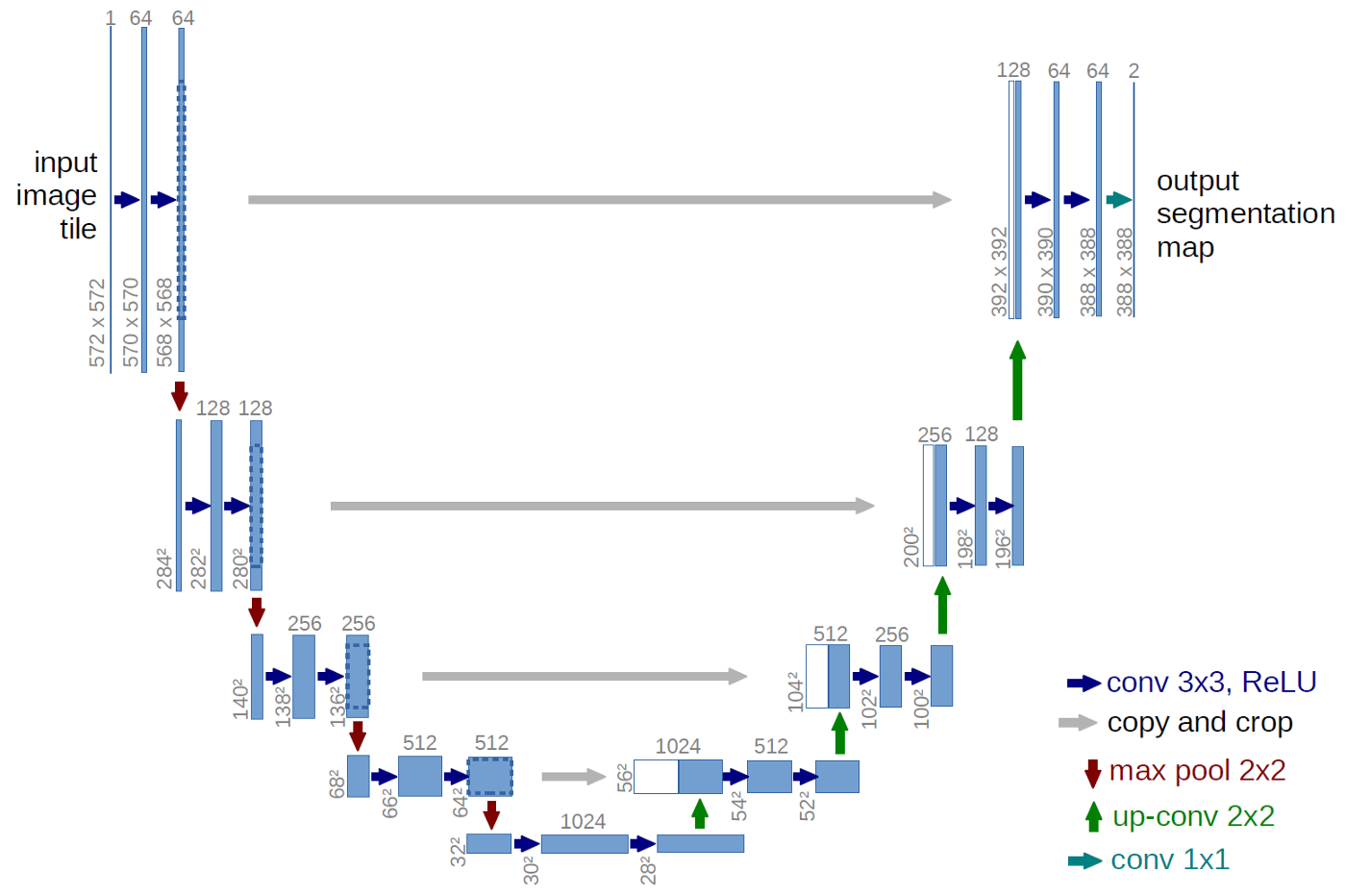
For U-Internet, actually an image says greater than many phrases:

Determine 2: U-Internet structure from Ronneberger et al. 2015.

At every upsampling stage we concatenate the output from the earlier layer with that from its counterpart within the compression stage. The ultimate output is a masks of dimension the unique picture, obtained through 1×1-convolution; no last dense layer is required, as an alternative the output layer is only a convolutional layer with a single filter.

Now let’s truly prepare a U-Internet. We’re going to make use of the unet bundle that allows you to create a well-performing mannequin in a single line:

remotes::install_github("r-tensorflow/unet")
library(unet)

# takes extra parameters, together with variety of downsizing blocks, 
# variety of filters to start out with, and variety of lessons to establish
# see ?unet for more information
mannequin <- unet(input_shape = c(128, 128, 3))

So we’ve got a mannequin, and it seems like we’ll be eager to feed it 128×128 RGB pictures. Now how can we get these pictures?

The info

As an instance how purposes come up even exterior the world of medical analysis, we’ll use for instance the Kaggle Carvana Picture Masking Problem. The duty is to create a segmentation masks separating automobiles from background. For our present goal, we solely want prepare.zip and train_mask.zip from the archive supplied for obtain. Within the following, we assume these have been extracted to a subdirectory referred to as data-raw.

Let’s first check out some pictures and their related segmentation masks.

The photographs are RGB-space JPEGs, whereas the masks are black-and-white GIFs.

We break up the info right into a coaching and a validation set. We’ll use the latter to watch generalization efficiency throughout coaching.

information <- tibble(
  img = record.information(right here::right here("data-raw/prepare"), full.names = TRUE),
  masks = record.information(right here::right here("data-raw/train_masks"), full.names = TRUE)
)

information <- initial_split(information, prop = 0.8)

To feed the info to the community, we’ll use tfdatasets. All preprocessing will find yourself in a easy pipeline, however we’ll first go over the required actions step-by-step.

Preprocessing pipeline

Step one is to learn within the pictures, making use of the suitable features in tf$picture.

training_dataset <- coaching(information) %>%  
  tensor_slices_dataset() %>% 
  dataset_map(~.x %>% list_modify(
    # decode_jpeg yields a 3d tensor of form (1280, 1918, 3)
    img = tf$picture$decode_jpeg(tf$io$read_file(.x$img)),
    # decode_gif yields a 4d tensor of form (1, 1280, 1918, 3),
    # so we take away the unneeded batch dimension and all however one 
    # of the three (an identical) channels
    masks = tf$picture$decode_gif(tf$io$read_file(.x$masks))[1,,,][,,1,drop=FALSE]
  ))

Whereas setting up a preprocessing pipeline, it’s very helpful to test intermediate outcomes.
It’s straightforward to do utilizing reticulate::as_iterator on the dataset:

$img
tf.Tensor(
[[[243 244 239]
  [243 244 239]
  [243 244 239]
  ...
 ...
  ...
  [175 179 178]
  [175 179 178]
  [175 179 178]]], form=(1280, 1918, 3), dtype=uint8)

$masks
tf.Tensor(
[[[0]
  [0]
  [0]
  ...
 ...
  ...
  [0]
  [0]
  [0]]], form=(1280, 1918, 1), dtype=uint8)

Whereas the uint8 datatype makes RGB values straightforward to learn for people, the community goes to count on floating level numbers. The next code converts its enter and moreover, scales values to the interval [0,1):

training_dataset <- training_dataset %>% 
  dataset_map(~.x %>% list_modify(
    img = tf$image$convert_image_dtype(.x$img, dtype = tf$float32),
    mask = tf$image$convert_image_dtype(.x$mask, dtype = tf$float32)
  ))

To reduce computational cost, we resize the images to size 128x128. This will change the aspect ratio and thus, distort the images, but is not a problem with the given dataset.

training_dataset <- training_dataset %>% 
  dataset_map(~.x %>% list_modify(
    img = tf$image$resize(.x$img, size = shape(128, 128)),
    mask = tf$image$resize(.x$mask, size = shape(128, 128))
  ))

Now, it’s well known that in deep learning, data augmentation is paramount. For segmentation, there’s one thing to consider, which is whether a transformation needs to be applied to the mask as well – this would be the case for e.g. rotations, or flipping. Here, results will be good enough applying just transformations that preserve positions:

random_bsh <- function(img) {
  img %>% 
    tf$image$random_brightness(max_delta = 0.3) %>% 
    tf$image$random_contrast(lower = 0.5, upper = 0.7) %>% 
    tf$image$random_saturation(lower = 0.5, upper = 0.7) %>% 
    # make sure we still are between 0 and 1
    tf$clip_by_value(0, 1) 
}

training_dataset <- training_dataset %>% 
  dataset_map(~.x %>% list_modify(
    img = random_bsh(.x$img)
  ))

Again, we can use as_iterator to see what these transformations do to our images:

Here’s the complete preprocessing pipeline.

create_dataset <- function(data, train, batch_size = 32L) {
  
  dataset <- data %>% 
    tensor_slices_dataset() %>% 
    dataset_map(~.x %>% list_modify(
      img = tf$image$decode_jpeg(tf$io$read_file(.x$img)),
      mask = tf$image$decode_gif(tf$io$read_file(.x$mask))[1,,,][,,1,drop=FALSE]
    )) %>% 
    dataset_map(~.x %>% list_modify(
      img = tf$picture$convert_image_dtype(.x$img, dtype = tf$float32),
      masks = tf$picture$convert_image_dtype(.x$masks, dtype = tf$float32)
    )) %>% 
    dataset_map(~.x %>% list_modify(
      img = tf$picture$resize(.x$img, dimension = form(128, 128)),
      masks = tf$picture$resize(.x$masks, dimension = form(128, 128))
    ))
  
  # information augmentation carried out on coaching set solely
  if (prepare) {
    dataset <- dataset %>% 
      dataset_map(~.x %>% list_modify(
        img = random_bsh(.x$img)
      )) 
  }
  
  # shuffling on coaching set solely
  if (prepare) {
    dataset <- dataset %>% 
      dataset_shuffle(buffer_size = batch_size*128)
  }
  
  # prepare in batches; batch dimension would possibly have to be tailored relying on
  # accessible reminiscence
  dataset <- dataset %>% 
    dataset_batch(batch_size)
  
  dataset %>% 
    # output must be unnamed
    dataset_map(unname) 
}

Coaching and check set creation now could be only a matter of two perform calls.

training_dataset <- create_dataset(coaching(information), prepare = TRUE)
validation_dataset <- create_dataset(testing(information), prepare = FALSE)

And we’re prepared to coach the mannequin.

Coaching the mannequin

We already confirmed the best way to create the mannequin, however let’s repeat it right here, and test mannequin structure:

mannequin <- unet(input_shape = c(128, 128, 3))
abstract(mannequin)

Mannequin: "mannequin"
______________________________________________________________________________________________
Layer (kind)                   Output Form        Param #    Related to                    
==============================================================================================
input_1 (InputLayer)           [(None, 128, 128, 3 0                                          
______________________________________________________________________________________________
conv2d (Conv2D)                (None, 128, 128, 64 1792       input_1[0][0]                   
______________________________________________________________________________________________
conv2d_1 (Conv2D)              (None, 128, 128, 64 36928      conv2d[0][0]                    
______________________________________________________________________________________________
max_pooling2d (MaxPooling2D)   (None, 64, 64, 64)  0          conv2d_1[0][0]                  
______________________________________________________________________________________________
conv2d_2 (Conv2D)              (None, 64, 64, 128) 73856      max_pooling2d[0][0]             
______________________________________________________________________________________________
conv2d_3 (Conv2D)              (None, 64, 64, 128) 147584     conv2d_2[0][0]                  
______________________________________________________________________________________________
max_pooling2d_1 (MaxPooling2D) (None, 32, 32, 128) 0          conv2d_3[0][0]                  
______________________________________________________________________________________________
conv2d_4 (Conv2D)              (None, 32, 32, 256) 295168     max_pooling2d_1[0][0]           
______________________________________________________________________________________________
conv2d_5 (Conv2D)              (None, 32, 32, 256) 590080     conv2d_4[0][0]                  
______________________________________________________________________________________________
max_pooling2d_2 (MaxPooling2D) (None, 16, 16, 256) 0          conv2d_5[0][0]                  
______________________________________________________________________________________________
conv2d_6 (Conv2D)              (None, 16, 16, 512) 1180160    max_pooling2d_2[0][0]           
______________________________________________________________________________________________
conv2d_7 (Conv2D)              (None, 16, 16, 512) 2359808    conv2d_6[0][0]                  
______________________________________________________________________________________________
max_pooling2d_3 (MaxPooling2D) (None, 8, 8, 512)   0          conv2d_7[0][0]                  
______________________________________________________________________________________________
dropout (Dropout)              (None, 8, 8, 512)   0          max_pooling2d_3[0][0]           
______________________________________________________________________________________________
conv2d_8 (Conv2D)              (None, 8, 8, 1024)  4719616    dropout[0][0]                   
______________________________________________________________________________________________
conv2d_9 (Conv2D)              (None, 8, 8, 1024)  9438208    conv2d_8[0][0]                  
______________________________________________________________________________________________
conv2d_transpose (Conv2DTransp (None, 16, 16, 512) 2097664    conv2d_9[0][0]                  
______________________________________________________________________________________________
concatenate (Concatenate)      (None, 16, 16, 1024 0          conv2d_7[0][0]                  
                                                              conv2d_transpose[0][0]          
______________________________________________________________________________________________
conv2d_10 (Conv2D)             (None, 16, 16, 512) 4719104    concatenate[0][0]               
______________________________________________________________________________________________
conv2d_11 (Conv2D)             (None, 16, 16, 512) 2359808    conv2d_10[0][0]                 
______________________________________________________________________________________________
conv2d_transpose_1 (Conv2DTran (None, 32, 32, 256) 524544     conv2d_11[0][0]                 
______________________________________________________________________________________________
concatenate_1 (Concatenate)    (None, 32, 32, 512) 0          conv2d_5[0][0]                  
                                                              conv2d_transpose_1[0][0]        
______________________________________________________________________________________________
conv2d_12 (Conv2D)             (None, 32, 32, 256) 1179904    concatenate_1[0][0]             
______________________________________________________________________________________________
conv2d_13 (Conv2D)             (None, 32, 32, 256) 590080     conv2d_12[0][0]                 
______________________________________________________________________________________________
conv2d_transpose_2 (Conv2DTran (None, 64, 64, 128) 131200     conv2d_13[0][0]                 
______________________________________________________________________________________________
concatenate_2 (Concatenate)    (None, 64, 64, 256) 0          conv2d_3[0][0]                  
                                                              conv2d_transpose_2[0][0]        
______________________________________________________________________________________________
conv2d_14 (Conv2D)             (None, 64, 64, 128) 295040     concatenate_2[0][0]             
______________________________________________________________________________________________
conv2d_15 (Conv2D)             (None, 64, 64, 128) 147584     conv2d_14[0][0]                 
______________________________________________________________________________________________
conv2d_transpose_3 (Conv2DTran (None, 128, 128, 64 32832      conv2d_15[0][0]                 
______________________________________________________________________________________________
concatenate_3 (Concatenate)    (None, 128, 128, 12 0          conv2d_1[0][0]                  
                                                              conv2d_transpose_3[0][0]        
______________________________________________________________________________________________
conv2d_16 (Conv2D)             (None, 128, 128, 64 73792      concatenate_3[0][0]             
______________________________________________________________________________________________
conv2d_17 (Conv2D)             (None, 128, 128, 64 36928      conv2d_16[0][0]                 
______________________________________________________________________________________________
conv2d_18 (Conv2D)             (None, 128, 128, 1) 65         conv2d_17[0][0]                 
==============================================================================================
Complete params: 31,031,745
Trainable params: 31,031,745
Non-trainable params: 0
______________________________________________________________________________________________

The “output form” column exhibits the anticipated U-shape numerically: Width and top first go down, till we attain a minimal decision of 8x8; they then go up once more, till we’ve reached the unique decision. On the similar time, the variety of filters first goes up, then goes down once more, till within the output layer we’ve got a single filter. You can even see the concatenate layers appending info that comes from “beneath” to info that comes “laterally.”

What needs to be the loss perform right here? We’re labeling every pixel, so every pixel contributes to the loss. We have now a binary downside – every pixel could also be “automotive” or “background” – so we wish every output to be near both 0 or 1. This makes binary_crossentropy the satisfactory loss perform.

Throughout coaching, we hold monitor of classification accuracy in addition to the cube coefficient, the analysis metric used within the competitors. The cube coefficient is a technique to measure the proportion of appropriate classifications:

cube <- custom_metric("cube", perform(y_true, y_pred, clean = 1.0) {
  y_true_f <- k_flatten(y_true)
  y_pred_f <- k_flatten(y_pred)
  intersection <- k_sum(y_true_f * y_pred_f)
  (2 * intersection + clean) / (k_sum(y_true_f) + k_sum(y_pred_f) + clean)
})

mannequin %>% compile(
  optimizer = optimizer_rmsprop(lr = 1e-5),
  loss = "binary_crossentropy",
  metrics = record(cube, metric_binary_accuracy)
)

Becoming the mannequin takes a while – how a lot, in fact, will rely in your {hardware}. However the wait pays off: After 5 epochs, we noticed a cube coefficient of ~ 0.87 on the validation set, and an accuracy of ~ 0.95.

Predictions

In fact, what we’re in the end all in favour of are predictions. Let’s see just a few masks generated for gadgets from the validation set:

batch <- validation_dataset %>% as_iterator() %>% iter_next()
predictions <- predict(mannequin, batch)

pictures <- tibble(
  picture = batch[[1]] %>% array_branch(1),
  predicted_mask = predictions[,,,1] %>% array_branch(1),
  masks = batch[[2]][,,,1]  %>% array_branch(1)
) %>% 
  sample_n(2) %>% 
  map_depth(2, perform(x) {
    as.raster(x) %>% magick::image_read()
  }) %>% 
  map(~do.name(c, .x))


out <- magick::image_append(c(
  magick::image_append(pictures$masks, stack = TRUE),
  magick::image_append(pictures$picture, stack = TRUE), 
  magick::image_append(pictures$predicted_mask, stack = TRUE)
  )
)

plot(out)

Determine 3: From left to proper: floor fact, enter picture, and predicted masks from U-Internet.

Conclusion

If there have been a contest for the very best sum of usefulness and architectural transparency, U-Internet would definitely be a contender. With out a lot tuning, it’s doable to acquire first rate outcomes. For those who’re in a position to put this mannequin to make use of in your work, or in case you have issues utilizing it, tell us! Thanks for studying!