Posit AI Weblog: Phrase Embeddings with Keras

Introduction

Phrase embedding is a technique used to map phrases of a vocabulary to
dense vectors of actual numbers the place semantically comparable phrases are mapped to
close by factors. Representing phrases on this vector area assist
algorithms obtain higher efficiency in pure language
processing duties like syntactic parsing and sentiment evaluation by grouping
comparable phrases. For instance, we count on that within the embedding area
“cats” and “canines” are mapped to close by factors since they’re
each animals, mammals, pets, and so forth.

On this tutorial we are going to implement the skip-gram mannequin created by Mikolov et al in R utilizing the keras package deal.
The skip-gram mannequin is a taste of word2vec, a category of
computationally-efficient predictive fashions for studying phrase
embeddings from uncooked textual content. We received’t deal with theoretical particulars about embeddings and
the skip-gram mannequin. If you wish to get extra particulars you possibly can learn the paper
linked above. The TensorFlow Vector Illustration of Phrases tutorial contains extra particulars as does the Deep Studying With R pocket book about embeddings.

There are different methods to create vector representations of phrases. For instance,
GloVe Embeddings are carried out within the text2vec package deal by Dmitriy Selivanov.
There’s additionally a tidy strategy described in Julia Silge’s weblog publish Phrase Vectors with Tidy Information Rules.

Getting the Information

We’ll use the Amazon High-quality Meals Critiques dataset.
This dataset consists of evaluations of positive meals from Amazon. The info span a interval of greater than 10 years, together with all ~500,000 evaluations as much as October 2012. Critiques embody product and consumer data, rankings, and narrative textual content.

Information could be downloaded (~116MB) by working:

obtain.file("https://snap.stanford.edu/information/finefoods.txt.gz", "finefoods.txt.gz")

We’ll now load the plain textual content evaluations into R.

Let’s check out some evaluations we’ve got within the dataset.

[1] "I've purchased a number of of the Vitality canned pet food merchandise ...
[2] "Product arrived labeled as Jumbo Salted Peanuts...the peanuts ... 

Preprocessing

We’ll start with some textual content pre-processing utilizing a keras text_tokenizer(). The tokenizer can be
answerable for remodeling every assessment right into a sequence of integer tokens (which can subsequently be used as
enter into the skip-gram mannequin).

library(keras)
tokenizer <- text_tokenizer(num_words = 20000)
tokenizer %>% fit_text_tokenizer(evaluations)

Be aware that the tokenizer object is modified in place by the decision to fit_text_tokenizer().
An integer token can be assigned for every of the 20,000 commonest phrases (the opposite phrases will
be assigned to token 0).

Skip-Gram Mannequin

Within the skip-gram mannequin we are going to use every phrase as enter to a log-linear classifier
with a projection layer, then predict phrases inside a sure vary earlier than and after
this phrase. It might be very computationally costly to output a likelihood
distribution over all of the vocabulary for every goal phrase we enter into the mannequin. As a substitute,
we’re going to use detrimental sampling, which means we are going to pattern some phrases that don’t
seem within the context and prepare a binary classifier to foretell if the context phrase we
handed is really from the context or not.

In additional sensible phrases, for the skip-gram mannequin we are going to enter a 1d integer vector of
the goal phrase tokens and a 1d integer vector of sampled context phrase tokens. We’ll
generate a prediction of 1 if the sampled phrase actually appeared within the context and 0 if it didn’t.

We’ll now outline a generator perform to yield batches for mannequin coaching.

library(reticulate)
library(purrr)
skipgrams_generator <- perform(textual content, tokenizer, window_size, negative_samples) {
  gen <- texts_to_sequences_generator(tokenizer, pattern(textual content))
  perform() {
    skip <- generator_next(gen) %>%
      skipgrams(
        vocabulary_size = tokenizer$num_words, 
        window_size = window_size, 
        negative_samples = 1
      )
    x <- transpose(skip${couples}) %>% map(. %>% unlist %>% as.matrix(ncol = 1))
    y <- skip$labels %>% as.matrix(ncol = 1)
    listing(x, y)
  }
}

A generator perform
is a perform that returns a special worth every time it’s known as (generator capabilities are sometimes used to supply streaming or dynamic information for coaching fashions). Our generator perform will obtain a vector of texts,
a tokenizer and the arguments for the skip-gram (the scale of the window round every
goal phrase we look at and what number of detrimental samples we would like
to pattern for every goal phrase).

Now let’s begin defining the keras mannequin. We’ll use the Keras purposeful API.

embedding_size <- 128  # Dimension of the embedding vector.
skip_window <- 5       # What number of phrases to think about left and proper.
num_sampled <- 1       # Variety of detrimental examples to pattern for every phrase.

We’ll first write placeholders for the inputs utilizing the layer_input perform.

input_target <- layer_input(form = 1)
input_context <- layer_input(form = 1)

Now let’s outline the embedding matrix. The embedding is a matrix with dimensions
(vocabulary, embedding_size) that acts as lookup desk for the phrase vectors.

embedding <- layer_embedding(
  input_dim = tokenizer$num_words + 1, 
  output_dim = embedding_size, 
  input_length = 1, 
  identify = "embedding"
)

target_vector <- input_target %>% 
  embedding() %>% 
  layer_flatten()

context_vector <- input_context %>%
  embedding() %>%
  layer_flatten()

The following step is to outline how the target_vector can be associated to the context_vector
in an effort to make our community output 1 when the context phrase actually appeared within the
context and 0 in any other case. We wish target_vector to be comparable to the context_vector
in the event that they appeared in the identical context. A typical measure of similarity is the cosine
similarity. Give two vectors (A) and (B)
the cosine similarity is outlined by the Euclidean Dot product of (A) and (B) normalized by their
magnitude. As we don’t want the similarity to be normalized contained in the community, we are going to solely calculate
the dot product after which output a dense layer with sigmoid activation.

dot_product <- layer_dot(listing(target_vector, context_vector), axes = 1)
output <- layer_dense(dot_product, models = 1, activation = "sigmoid")

Now we are going to create the mannequin and compile it.

mannequin <- keras_model(listing(input_target, input_context), output)
mannequin %>% compile(loss = "binary_crossentropy", optimizer = "adam")

We are able to see the total definition of the mannequin by calling abstract:

_________________________________________________________________________________________
Layer (kind)                 Output Form       Param #    Related to                  
=========================================================================================
input_1 (InputLayer)         (None, 1)          0                                        
_________________________________________________________________________________________
input_2 (InputLayer)         (None, 1)          0                                        
_________________________________________________________________________________________
embedding (Embedding)        (None, 1, 128)     2560128    input_1[0][0]                 
                                                           input_2[0][0]                 
_________________________________________________________________________________________
flatten_1 (Flatten)          (None, 128)        0          embedding[0][0]               
_________________________________________________________________________________________
flatten_2 (Flatten)          (None, 128)        0          embedding[1][0]               
_________________________________________________________________________________________
dot_1 (Dot)                  (None, 1)          0          flatten_1[0][0]               
                                                           flatten_2[0][0]               
_________________________________________________________________________________________
dense_1 (Dense)              (None, 1)          2          dot_1[0][0]                   
=========================================================================================
Complete params: 2,560,130
Trainable params: 2,560,130
Non-trainable params: 0
_________________________________________________________________________________________

Mannequin Coaching

We’ll match the mannequin utilizing the fit_generator() perform We have to specify the variety of
coaching steps in addition to variety of epochs we need to prepare. We’ll prepare for
100,000 steps for five epochs. That is fairly sluggish (~1000 seconds per epoch on a contemporary GPU). Be aware that you simply
may additionally get cheap outcomes with only one epoch of coaching.

mannequin %>%
  fit_generator(
    skipgrams_generator(evaluations, tokenizer, skip_window, negative_samples), 
    steps_per_epoch = 100000, epochs = 5
    )

Epoch 1/1
100000/100000 [==============================] - 1092s - loss: 0.3749      
Epoch 2/5
100000/100000 [==============================] - 1094s - loss: 0.3548     
Epoch 3/5
100000/100000 [==============================] - 1053s - loss: 0.3630     
Epoch 4/5
100000/100000 [==============================] - 1020s - loss: 0.3737     
Epoch 5/5
100000/100000 [==============================] - 1017s - loss: 0.3823 

We are able to now extract the embeddings matrix from the mannequin through the use of the get_weights()
perform. We additionally added row.names to our embedding matrix so we will simply discover
the place every phrase is.

Understanding the Embeddings

We are able to now discover phrases which are shut to one another within the embedding. We’ll
use the cosine similarity, since that is what we educated the mannequin to
reduce.

library(text2vec)

find_similar_words <- perform(phrase, embedding_matrix, n = 5) {
  similarities <- embedding_matrix[word, , drop = FALSE] %>%
    sim2(embedding_matrix, y = ., methodology = "cosine")
  
  similarities[,1] %>% kind(reducing = TRUE) %>% head(n)
}

find_similar_words("2", embedding_matrix)

        2         4         3       two         6 
1.0000000 0.9830254 0.9777042 0.9765668 0.9722549 

find_similar_words("little", embedding_matrix)

   little       bit       few     small     deal with 
1.0000000 0.9501037 0.9478287 0.9309829 0.9286966 

find_similar_words("scrumptious", embedding_matrix)

scrumptious     tasty great   wonderful     yummy 
1.0000000 0.9632145 0.9619508 0.9617954 0.9529505 

find_similar_words("cats", embedding_matrix)

     cats      canines      youngsters       cat       canine 
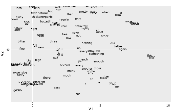
1.0000000 0.9844937 0.9743756 0.9676026 0.9624494 

The t-SNE algorithm can be utilized to visualise the embeddings. Due to time constraints we
will solely use it with the primary 500 phrases. To grasp extra in regards to the t-SNE methodology see the article The way to Use t-SNE Successfully.

This plot could appear to be a multitude, however if you happen to zoom into the small teams you find yourself seeing some good patterns.
Strive, for instance, to discover a group of net associated phrases like http, href, and so forth. One other group
that could be simple to pick is the pronouns group: she, he, her, and so forth.