
How would your summer season vacation’s pictures look had Edvard Munch painted them? (Maybe it’s higher to not know).
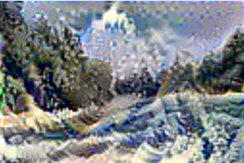
Let’s take a extra comforting instance: How would a pleasant, summarly river panorama look if painted by Katsushika Hokusai?
Model switch on photos is just not new, however obtained a lift when Gatys, Ecker, and Bethge(Gatys, Ecker, and Bethge 2015) confirmed easy methods to efficiently do it with deep studying.
The principle thought is easy: Create a hybrid that could be a tradeoff between the content material picture we wish to manipulate, and a fashion picture we wish to imitate, by optimizing for maximal resemblance to each on the identical time.
When you’ve learn the chapter on neural fashion switch from Deep Studying with R, chances are you’ll acknowledge a number of the code snippets that observe.
Nevertheless, there is a vital distinction: This submit makes use of TensorFlow Keen Execution, permitting for an crucial means of coding that makes it simple to map ideas to code.
Similar to earlier posts on keen execution on this weblog, this can be a port of a Google Colaboratory pocket book that performs the identical job in Python.
As normal, please be sure you have the required package deal variations put in. And no want to repeat the snippets – you’ll discover the whole code among the many Keras examples.
Conditions
The code on this submit is determined by the newest variations of a number of of the TensorFlow R packages. You possibly can set up these packages as follows:

And right here’s the fashion mannequin, Hokusai’s The Nice Wave off Kanagawa, which you’ll be able to obtain from Wikimedia Commons:

We create a wrapper that hundreds and preprocesses the enter photos for us.
As we shall be working with VGG19, a community that has been educated on ImageNet, we have to rework our enter photos in the identical means that was used coaching it. Later, we’ll apply the inverse transformation to our mixture picture earlier than displaying it.
load_and_preprocess_image <- perform(path) {
  img <- image_load(path, target_size = img_shape[1:2]) %>%
    image_to_array() %>%
    k_expand_dims(axis = 1) %>%
    imagenet_preprocess_input()
}

deprocess_image <- perform(x) {
  x <- x[1, , ,]
  # Take away zero-center by imply pixel
  x[, , 1] <- x[, , 1] + 103.939
  x[, , 2] <- x[, , 2] + 116.779
  x[, , 3] <- x[, , 3] + 123.68
  # 'BGR'->'RGB'
  x <- x[, , c(3, 2, 1)]
  x[x > 255] <- 255
  x[x < 0] <- 0
  x[] <- as.integer(x) / 255
  x
}
Setting the scene
We’re going to use a neural community, however we gained’t be coaching it. Neural fashion switch is a bit unusual in that we don’t optimize the community’s weights, however again propagate the loss to the enter layer (the picture), as a way to transfer it within the desired course.
We shall be considering two sorts of outputs from the community, comparable to our two targets.
Firstly, we wish to hold the mix picture much like the content material picture, on a excessive stage. In a convnet, higher layers map to extra holistic ideas, so we’re selecting a layer excessive up within the graph to check outputs from the supply and the mix.
Secondly, the generated picture ought to “appear like” the fashion picture. Model corresponds to decrease stage options like texture, shapes, strokes… So to check the mix towards the fashion instance, we select a set of decrease stage conv blocks for comparability and mixture the outcomes.
content_layers <- c("block5_conv2")
style_layers <- c("block1_conv1",
                 "block2_conv1",
                 "block3_conv1",
                 "block4_conv1",
                 "block5_conv1")

num_content_layers <- size(content_layers)
num_style_layers <- size(style_layers)

get_model <- perform() {
  vgg <- application_vgg19(include_top = FALSE, weights = "imagenet")
  vgg$trainable <- FALSE
  style_outputs <- map(style_layers, perform(layer) vgg$get_layer(layer)$output)
  content_outputs <- map(content_layers, perform(layer) vgg$get_layer(layer)$output)
  model_outputs <- c(style_outputs, content_outputs)
  keras_model(vgg$enter, model_outputs)
}
Losses
When optimizing the enter picture, we’ll think about three sorts of losses. Firstly, the content material loss: How completely different is the mix picture from the supply? Right here, we’re utilizing the sum of the squared errors for comparability.
content_loss <- perform(content_image, goal) {
  k_sum(k_square(goal - content_image))
}
Our second concern is having the kinds match as carefully as potential. Model is often operationalized because the Gram matrix of flattened characteristic maps in a layer. We thus assume that fashion is expounded to how maps in a layer correlate with different.
We subsequently compute the Gram matrices of the layers we’re considering (outlined above), for the supply picture in addition to the optimization candidate, and evaluate them, once more utilizing the sum of squared errors.
gram_matrix <- perform(x) {
  options <- k_batch_flatten(k_permute_dimensions(x, c(3, 1, 2)))
  gram <- k_dot(options, k_transpose(options))
  gram
}

style_loss <- perform(gram_target, mixture) {
  gram_comb <- gram_matrix(mixture)
  k_sum(k_square(gram_target - gram_comb)) /
    (4 * (img_shape[3] ^ 2) * (img_shape[1] * img_shape[2]) ^ 2)
}
Thirdly, we don’t need the mix picture to look overly pixelated, thus we’re including in a regularization element, the overall variation within the picture:
total_variation_loss <- perform(picture) {
  y_ij  <- picture[1:(img_shape[1] - 1L), 1:(img_shape[2] - 1L),]
  y_i1j <- picture[2:(img_shape[1]), 1:(img_shape[2] - 1L),]
  y_ij1 <- picture[1:(img_shape[1] - 1L), 2:(img_shape[2]),]
  a <- k_square(y_ij - y_i1j)
  b <- k_square(y_ij - y_ij1)
  k_sum(k_pow(a + b, 1.25))
}
The difficult factor is easy methods to mix these losses. We’ve reached acceptable outcomes with the next weightings, however be happy to mess around as you see match:
content_weight <- 100
style_weight <- 0.8
total_variation_weight <- 0.01
Get mannequin outputs for the content material and elegance photos
We’d like the mannequin’s output for the content material and elegance photos, however right here it suffices to do that simply as soon as.
We concatenate each photos alongside the batch dimension, cross that enter to the mannequin, and get again a listing of outputs, the place each aspect of the listing is a 4-d tensor. For the fashion picture, we’re within the fashion outputs at batch place 1, whereas for the content material picture, we’d like the content material output at batch place 2.
Within the beneath feedback, please be aware that the sizes of dimensions 2 and three will differ if you happen to’re loading photos at a distinct dimension.
get_feature_representations <-
  perform(mannequin, content_path, style_path) {

    # dim == (1, 128, 128, 3)
    style_image <-
      load_and_process_image(style_path) %>% k_cast("float32")
    # dim == (1, 128, 128, 3)
    content_image <-
      load_and_process_image(content_path) %>% k_cast("float32")
    # dim == (2, 128, 128, 3)
    stack_images <- k_concatenate(listing(style_image, content_image), axis = 1)

    # size(model_outputs) == 6
    # dim(model_outputs[[1]]) = (2, 128, 128, 64)
    # dim(model_outputs[[6]]) = (2, 8, 8, 512)
    model_outputs <- mannequin(stack_images)

    style_features <-
      model_outputs[1:num_style_layers] %>%
      map(perform(batch) batch[1, , , ])
    content_features <-
      model_outputs[(num_style_layers + 1):(num_style_layers + num_content_layers)] %>%
      map(perform(batch) batch[2, , , ])

    listing(style_features, content_features)
  }
Computing the losses
On each iteration, we have to cross the mix picture via the mannequin, receive the fashion and content material outputs, and compute the losses. Once more, the code is extensively commented with tensor sizes for straightforward verification, however please remember the fact that the precise numbers presuppose you’re working with 128×128 photos.
compute_loss <-
  perform(mannequin, loss_weights, init_image, gram_style_features, content_features) {

    c(style_weight, content_weight) %<-% loss_weights
    model_outputs <- mannequin(init_image)
    style_output_features <- model_outputs[1:num_style_layers]
    content_output_features <-
      model_outputs[(num_style_layers + 1):(num_style_layers + num_content_layers)]

    # fashion loss
    weight_per_style_layer <- 1 / num_style_layers
    style_score <- 0
    # dim(style_zip[[5]][[1]]) == (512, 512)
    style_zip <- transpose(listing(gram_style_features, style_output_features))
    for (l in 1:size(style_zip)) {
      # for l == 1:
      # dim(target_style) == (64, 64)
      # dim(comb_style) == (1, 128, 128, 64)
      c(target_style, comb_style) %<-% style_zip[[l]]
      style_score <- style_score + weight_per_style_layer *
        style_loss(target_style, comb_style[1, , , ])
    }

    # content material loss
    weight_per_content_layer <- 1 / num_content_layers
    content_score <- 0
    content_zip <- transpose(listing(content_features, content_output_features))
    for (l in 1:size(content_zip)) {
      # dim(comb_content) ==  (1, 8, 8, 512)
      # dim(target_content) == (8, 8, 512)
      c(target_content, comb_content) %<-% content_zip[[l]]
      content_score <- content_score + weight_per_content_layer *
        content_loss(comb_content[1, , , ], target_content)
    }

    # whole variation loss
    variation_loss <- total_variation_loss(init_image[1, , ,])

    style_score <- style_score * style_weight
    content_score <- content_score * content_weight
    variation_score <- variation_loss * total_variation_weight

    loss <- style_score + content_score + variation_score
    listing(loss, style_score, content_score, variation_score)
  }
Computing the gradients
As quickly as we now have the losses, acquiring the gradients of the general loss with respect to the enter picture is only a matter of calling tape$gradient on the GradientTape. Be aware that the nested name to compute_loss, and thus the decision of the mannequin on our mixture picture, occurs contained in the GradientTape context.
compute_grads <-
  perform(mannequin, loss_weights, init_image, gram_style_features, content_features) {
    with(tf$GradientTape() %as% tape, {
      scores <-
        compute_loss(mannequin,
                     loss_weights,
                     init_image,
                     gram_style_features,
                     content_features)
    })
    total_loss <- scores[[1]]
    listing(tape$gradient(total_loss, init_image), scores)
  }
Coaching part
Now it’s time to coach! Whereas the pure continuation of this sentence would have been “… the mannequin,” the mannequin we’re coaching right here is just not VGG19 (that one we’re simply utilizing as a instrument), however a minimal setup of simply:
- a
Variablethat holds our to-be-optimized picture - the loss features we outlined above
- an optimizer that can apply the calculated gradients to the picture variable (
tf$practice$AdamOptimizer)
Under, we get the fashion options (of the fashion picture) and the content material characteristic (of the content material picture) simply as soon as, then iterate over the optimization course of, saving the output each 100 iterations.
In distinction to the unique article and the Deep Studying with R e book, however following the Google pocket book as a substitute, we’re not utilizing L-BFGS for optimization, however Adam, as our objective right here is to supply a concise introduction to keen execution.
Nevertheless, you would plug in one other optimization methodology if you happen to needed, changing
optimizer$apply_gradients(listing(tuple(grads, init_image)))
by an algorithm of your selection (and naturally, assigning the results of the optimization to the Variable holding the picture).
run_style_transfer <- perform(content_path, style_path) {
  mannequin <- get_model()
  stroll(mannequin$layers, perform(layer) layer$trainable = FALSE)

  c(style_features, content_features) %<-%
    get_feature_representations(mannequin, content_path, style_path)
  # dim(gram_style_features[[1]]) == (64, 64)
  gram_style_features <- map(style_features, perform(characteristic) gram_matrix(characteristic))

  init_image <- load_and_process_image(content_path)
  init_image <- tf$contrib$keen$Variable(init_image, dtype = "float32")

  optimizer <- tf$practice$AdamOptimizer(learning_rate = 1,
                                      beta1 = 0.99,
                                      epsilon = 1e-1)

  c(best_loss, best_image) %<-% listing(Inf, NULL)
  loss_weights <- listing(style_weight, content_weight)

  start_time <- Sys.time()
  global_start <- Sys.time()

  norm_means <- c(103.939, 116.779, 123.68)
  min_vals <- -norm_means
  max_vals <- 255 - norm_means

  for (i in seq_len(num_iterations)) {
    # dim(grads) == (1, 128, 128, 3)
    c(grads, all_losses) %<-% compute_grads(mannequin,
                                            loss_weights,
                                            init_image,
                                            gram_style_features,
                                            content_features)
    c(loss, style_score, content_score, variation_score) %<-% all_losses
    optimizer$apply_gradients(listing(tuple(grads, init_image)))
    clipped <- tf$clip_by_value(init_image, min_vals, max_vals)
    init_image$assign(clipped)

    end_time <- Sys.time()

    if (k_cast_to_floatx(loss) < best_loss) {
      best_loss <- k_cast_to_floatx(loss)
      best_image <- init_image
    }

    if (i %% 50 == 0) {
      glue("Iteration: {i}") %>% print()
      glue(
        "Complete loss: {k_cast_to_floatx(loss)},
        fashion loss: {k_cast_to_floatx(style_score)},
        content material loss: {k_cast_to_floatx(content_score)},
        whole variation loss: {k_cast_to_floatx(variation_score)},
        time for 1 iteration: {(Sys.time() - start_time) %>% spherical(2)}"
      ) %>% print()

      if (i %% 100 == 0) {
        png(paste0("style_epoch_", i, ".png"))
        plot_image <- best_image$numpy()
        plot_image <- deprocess_image(plot_image)
        plot(as.raster(plot_image), principal = glue("Iteration {i}"))
        dev.off()
      }
    }
  }

  glue("Complete time: {Sys.time() - global_start} seconds") %>% print()
  listing(best_image, best_loss)
}
Able to run
Now, we’re prepared to begin the method:
c(best_image, best_loss) %<-% run_style_transfer(content_path, style_path)In our case, outcomes didn’t change a lot after ~ iteration 1000, and that is how our river panorama was wanting:

… undoubtedly extra inviting than had it been painted by Edvard Munch!
Conclusion
With neural fashion switch, some fiddling round could also be wanted till you get the outcome you need. However as our instance exhibits, this doesn’t imply the code must be difficult. Moreover to being simple to know, keen execution additionally allows you to add debugging output, and step via the code line-by-line to test on tensor shapes.
Till subsequent time in our keen execution collection!
