Knowledge Preprocessing in R – GeeksforGeeks

Welcome, adventurous knowledge fanatics! At this time we have a good time an thrilling journey full of plenty of twists, turns, and enjoyable, as we dive into the world of information cleansing and visualization by way of R Programming Language. Seize your digital backpacks, put in your knowledge detective hats, Able to unravel the secrets and techniques of a dataset full of check outcomes and fascinating options.

Knowledge Preprocessing in R

Putting in and loading the tidyverse bundle.

The Tidyverse Metapackage – Our journey begins with the mysterious meta-package referred to as “tidyverse.” With a easy incantation, “library(tidyverse)” we unlock the highly effective instruments and unleash the magic of information manipulation and visualization.

Itemizing recordsdata within the “../enter” listing.

As we discover additional, we encounter a mystical listing often called “../enter/”. With a flick of our code wand, we unleash its secrets and techniques and reveal an inventory of hidden recordsdata.

── Attaching core tidyverse packages ──────────────────────── tidyverse 2.0.0 ──
✔ dplyr     1.1.2     ✔ readr     2.1.4
✔ forcats   1.0.0     ✔ stringr   1.5.0
✔ ggplot2   3.4.2     ✔ tibble    3.2.1
✔ lubridate 1.9.2     ✔ tidyr     1.3.0
✔ purrr     1.0.1     
── Conflicts ────────────────────────────────────────── tidyverse_conflicts() ──
✖ dplyr::filter() masks stats::filter()
✖ dplyr::lag()    masks stats::lag()
ℹ Use the conflicted bundle (<http://conflicted.r-lib.org/>) to drive all conflicts to develop into errors

The Magical Powers of “psych“, we encounter a uncommon gem often called “psych.” With, “set up.packages(‘psych’)” adopted by “library(psych),” we unlock its potent skills.

Studying the Dataset

We stumbled upon a treasured artifact—a CSV file named “Expanded_data_with_more_features.csv“. With a wave of our wand and the invocation of “learn.csv()“, we summon the information into our realm.

Knowledge Exploration & Evaluation

Our journey begins with a easy process—discovering what lies inside our dataset. We load the information and take a sneak peek. With the “head()” operate, we unveil the primary 5 rows. We revel within the pleasure of exploring the scale of our dataset utilizing “dim()“.

Output:

30641 * 15

You’ve summoned the names() operate to disclose the key names of the columns in your dataset. By capturing the output within the variable variable_names and invoking the print() spell, you have got efficiently unveiled the hidden names of the columns, permitting you to grasp the construction of your dataset.

Output:

 [1] "X"                   "Gender"              "EthnicGroup"        
 [4] "ParentEduc"          "LunchType"           "TestPrep"           
 [7] "ParentMaritalStatus" "PracticeSport"       "IsFirstChild"       
[10] "NrSiblings"          "TransportMeans"      "WklyStudyHours"     
[13] "MathScore"           "ReadingScore"        "WritingScore" 

Subsequent, you forged the str() spell upon your dataset. This spell reveals the information sorts of every variable (column) granting you perception into their mystical nature. By deciphering the output of this spell, you possibly can perceive the sorts of variables current in your dataset, resembling character (chr) numeric (num), or components, amongst others.

Output:

'knowledge.body':    30641 obs. of  15 variables:
 $ X                  : int  0 1 2 3 4 5 6 7 8 9 ...
 $ Gender             : chr  "feminine" "feminine" "feminine" "male" ...
 $ EthnicGroup        : chr  "" "group C" "group B" "group A" ...
 $ ParentEduc         : chr  "bachelor's diploma" "some faculty" "grasp's diploma"
                          "affiliate's diploma" ...
 $ LunchType          : chr  "normal" "normal" "normal" "free/diminished" ...
 $ TestPrep           : chr  "none" "" "none" "none" ...
 $ ParentMaritalStatus: chr  "married" "married" "single" "married" ...
 $ PracticeSport      : chr  "usually" "generally" "generally" "by no means" ...
 $ IsFirstChild       : chr  "sure" "sure" "sure" "no" ...
 $ NrSiblings         : int  3 0 4 1 0 1 1 1 3 NA ...
 $ TransportMeans     : chr  "school_bus" "" "school_bus" "" ...
 $ WklyStudyHours     : chr  "< 5" "5 - 10" "< 5" "5 - 10" ...
 $ MathScore          : int  71 69 87 45 76 73 85 41 65 37 ...
 $ ReadingScore       : int  71 90 93 56 78 84 93 43 64 59 ...
 $ WritingScore       : int  74 88 91 42 75 79 89 39 68 50 ...

Ah, however wait! Your eager eyes have noticed an anomaly. The variable “WklyStudyHours” seems to have been labeled as a personality (chr) as a substitute of its rightful numeric (num) nature. Concern not, for you possess the facility to appropriate this. To rectify this discrepancy, you need to use knowledge$WklyStudy…….. Ooopz can’t join with the spell hold exploring the journey see within the subsequent half hahaha hahaha hahaha  

Knowledge Cleansing & Formatting

The Magical Transformation Ah, However our dataset has just a few quirks, like lacking values and undesirable index columns. Concern not, With a splash of code, we bid farewell to the additional index column and wave our wands to transform clean areas into the magical realm of NA values. Step-by-step, we breathe life into our dataset, making certain every column shines brightly with the proper knowledge kind.

Dealing with Lacking Values

A World of Lacking Values Ahoy! We’ve stumbled upon lacking values! However fret not, we will fill these gaps and restore stability to our dataset. One after the other, we rescue columns from the clutches of vacancy, changing the void with the commonest classes. The lacking values tremble as we conquer them, remodeling our dataset into an entire and harmonious entity.

Output:

Gender:0
EthnicGroup:1840
ParentEduc:1845
LunchType:0
TestPrep:1830
ParentMaritalStatus:1190
PracticeSport:631
IsFirstChild:904
NrSiblings:1572
TransportMeans:3134
WklyStudyHours:0
MathScore:0
ReadingScore:0
WritingScore:0

Dealing with Categorical Knowledge

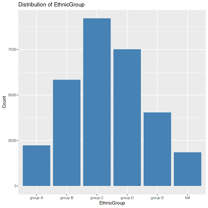
Unveiling the Secrets and techniques of Categorical Columns. Let’s begin with the EthnicGroup column first because it has 1840 lacking values.

Output:

NA 'group C' 'group B' 'group A' 'group D' 'group E'

Output:

Output:

[1] "group C"

Output:

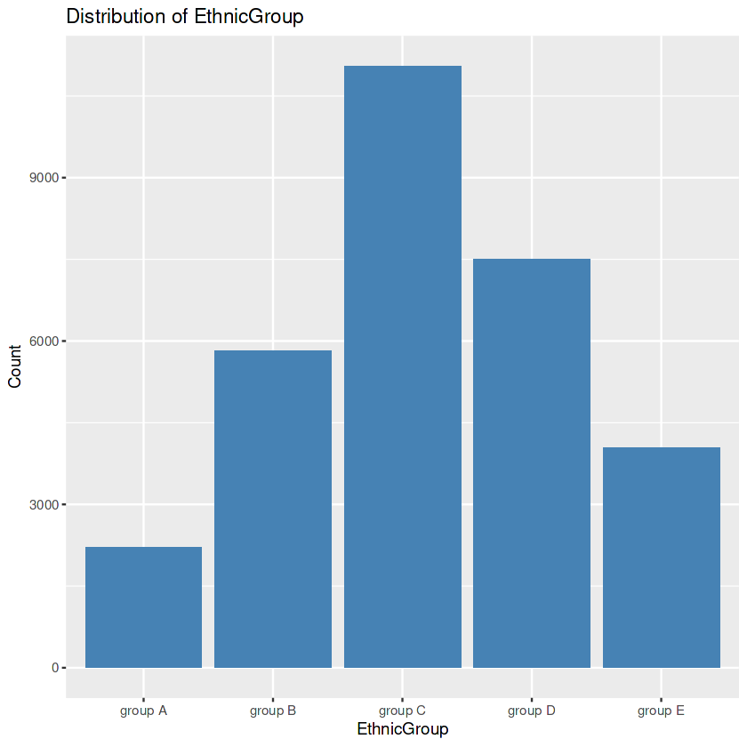
First, we search the exact values inside the “EthnicGroup” to find the superior ethnic teams current in our dataset. Then we create a bar plot. After this, we calculate the frequency rely for each class. This step permits us to grasp the distribution of ethnic firms additional quantitatively. We then determine the category with the best rely. Within the occasion of missing values inside the “EthnicGroup” column, we tackle this issue by the use of filling those gaps with the mode’s price. Lastly, we create one other bar plot of the “EthnicGroup” column, this time after eliminating the lacking values. The visualization serves as a distinction to the previous plot.

By executing the under code block we can impute the lacking values within the ParentEduc, WklyStudyHours, and NrSiblings.

Now we are going to use just a little bit refined methodology to fill within the lacking values within the remaining columns of the information.

Now let’s examine whether or not there are any extra lacking values left within the dataset or not.

Output:

0

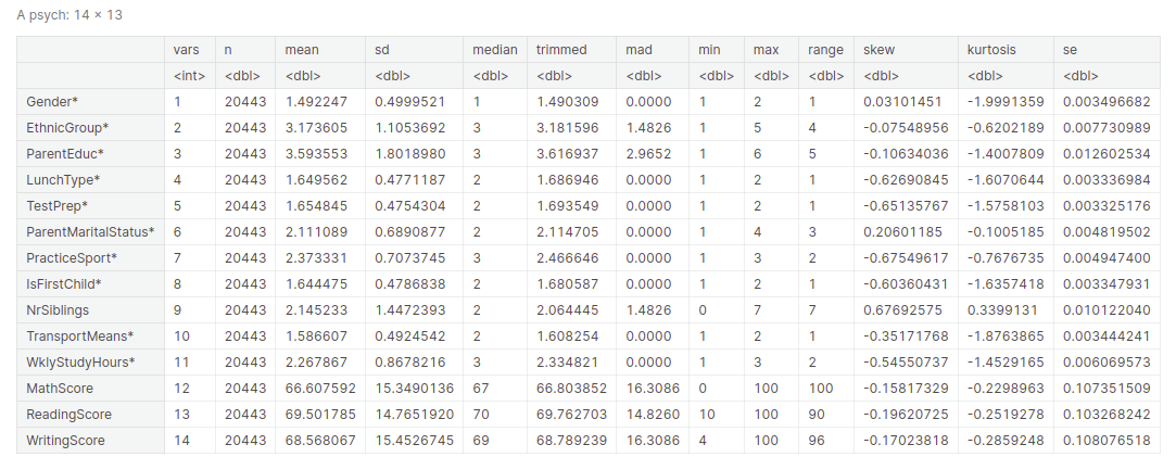
Descriptive statistical measures of a dataset assist us higher visualize and discover the dataset at hand with out going by way of every commentary of the dataset. We will get all of the descriptive statistical measures of the dataset utilizing the describe() operate.

Output:

Characteristic scaling

There are occasions when we now have completely different options within the dataset on completely different scales. So, whereas utilizing the gradient descent algorithm for coaching of the Machine Studying Algorithms it’s suggested to make use of options that are on the identical scale to have steady and quick coaching of our algorithm. There are completely different strategies of function scaling like standardization and normalization which is often known as Min-Max Scaling.

Standardization

Standardizing is like giving your stats a change! Think about you have got a bunch of buddies, all of whom are of various heights and weights. Some are lengthy, some are heavy, tough to check straight. So what do you guys do? You deliver a magic tailor with their requirements! The tailor takes every good friend and measures their peak and weight. Then, these measurements are transformed to a brand new scale the place every individual’s peak and weight are adjusted to equal imply and worth. Now, all your pals are “standardized” in a technique. Modified for ease of comparability and evaluation.

Thus, standardization is all about changing knowledge to a typical scale to facilitate comparability and evaluation. It’s like giving your stats a modern makeover to disclose their true magnificence and energy!

1. Create a brand new dataframe standardized_data as a replica of the unique knowledge dataframe.
2. Standardize the MathScore column in standardized_data utilizing the size() operate.
3. Print the primary few standardized values of MathScore utilizing head().

Output:

           [,1]
[1,]  0.2758342
[2,]  1.3395404
[3,]  0.6082424
[4,]  0.4087975
[5,]  1.2065771
[6,] -1.7186149

Normalization

Normalization is like giving your info a makeover to make them first-class! It’s like dressing up your numbers and making them sense assured and pleasing. Identical to getting every individual to placed on the same-sized t-shirt, normalization adjusts the values so all of them match correctly inside a specific vary(0-1). It’s like bringing concord to your statistics, making it simpler to look at and analyze. So, let’s get your info outfitted to shine with some normalization magic!

• Create a brand new dataframe normalized_data as a replica of the unique knowledge.
• Normalize the values within the MathScore column utilizing the system:

(normalized_data$MathScore - min(normalized_data$MathScore)) / (max(normalized_data$MathScore) - min(normalized_data$MathScore)).

• The normalized MathScore values are saved within the variable normalized_math, starting from 0 to 1

Output:

0.71 0.87 0.76 0.73 0.85 0.41

Characteristic Encoding

Characteristic encoding is like instructing your knowledge to talk the identical language as your pc. It’s like giving your knowledge a crash course in communications. Characteristic encoding is a way for changing categorical or non-numeric knowledge right into a numeric illustration .

One Sizzling Encoding

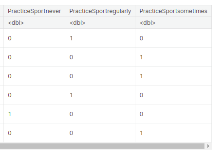
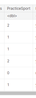
One Sizzling encoding is a approach to signify categorical variables as numeric values. We’re creating a brand new knowledge body referred to as “encoded_data” utilizing one-hot encoding for the “PracticeSport” variable.

1. Every distinctive worth within the “PracticeSport” column is remodeled right into a separate column with binary values (0s and 1s) indicating the presence or absence of that worth.
2. The unique knowledge body “knowledge” is mixed with the encoded columns utilizing the “cbind” operate, ensuing within the new “encoded_data” knowledge body.

Output:

Ordinal encoding

1. Ordinal encoding is used to signify categorical variables with ordered or hierarchical relationships utilizing numerical values.
2. Within the case of the “PracticeSport” column, we assigned numerical values to the classes “by no means”, “generally”, and “usually” based mostly on their order. “by no means” was assigned 0, “generally” was assigned 1, and “usually” was assigned 2.

Output:

Dealing with outliers

Field Plots: The Guardians of Numerical Columns – MathScore, ReadingScore, and WritingScore—maintain untold tales inside. However behold, outliers lurk within the shadows, threatening to skew our insights. Concern not, for we summon the facility of field plots to conquer these outliers and restore stability to our numerical realm.

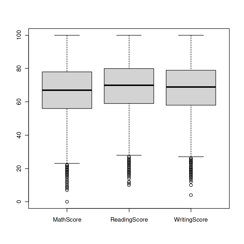
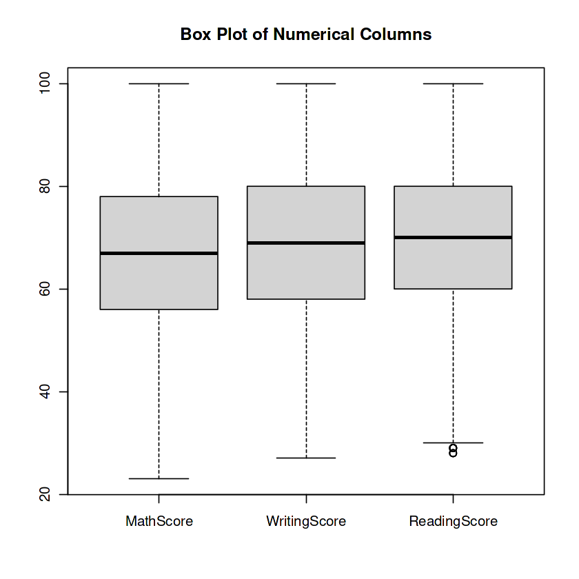
The code calculates the bounds for outlier detection in a number of columns of the knowledge dataframe. It then eliminates the outliers from every column and creates a field plot. This permits to find and address outliers inside the information.

Output:

And that’s a wrap! However keep in mind, that is just the start of our knowledge journey. There’s an enormous world of research, modeling, and interpretation awaiting us. So gear up, maintain on tight, and let’s proceed unraveling the mysteries hidden inside the knowledge!

Hold exploring and have enjoyable in your data-driven escapades!