Deep Studying for Textual content Classification with Keras

The IMDB dataset

On this instance, we’ll work with the IMDB dataset: a set of fifty,000 extremely polarized critiques from the Web Film Database. They’re cut up into 25,000 critiques for coaching and 25,000 critiques for testing, every set consisting of fifty% unfavorable and 50% optimistic critiques.

Why use separate coaching and take a look at units? Since you ought to by no means take a look at a machine-learning mannequin on the identical information that you simply used to coach it! Simply because a mannequin performs effectively on its coaching information doesn’t imply it’ll carry out effectively on information it has by no means seen; and what you care about is your mannequin’s efficiency on new information (since you already know the labels of your coaching information – clearly
you don’t want your mannequin to foretell these). For example, it’s potential that your mannequin may find yourself merely memorizing a mapping between your coaching samples and their targets, which might be ineffective for the duty of predicting targets for information the mannequin has by no means seen earlier than. We’ll go over this level in way more element within the subsequent chapter.

Identical to the MNIST dataset, the IMDB dataset comes packaged with Keras. It has already been preprocessed: the critiques (sequences of phrases) have been was sequences of integers, the place every integer stands for a particular phrase in a dictionary.

The next code will load the dataset (while you run it the primary time, about 80 MB of knowledge shall be downloaded to your machine).

library(keras)
imdb <- dataset_imdb(num_words = 10000)
train_data <- imdb$practice$x
train_labels <- imdb$practice$y
test_data <- imdb$take a look at$x
test_labels <- imdb$take a look at$y

The argument num_words = 10000 means you’ll solely maintain the highest 10,000 most ceaselessly occurring phrases within the coaching information. Uncommon phrases shall be discarded. This lets you work with vector information of manageable dimension.

The variables train_data and test_data are lists of critiques; every assessment is an inventory of phrase indices (encoding a sequence of phrases). train_labels and test_labels are lists of 0s and 1s, the place 0 stands for unfavorable and 1 stands for optimistic:

int [1:218] 1 14 22 16 43 530 973 1622 1385 65 ...

[1] 1

Since you’re proscribing your self to the highest 10,000 most frequent phrases, no phrase index will exceed 10,000:

[1] 9999

For kicks, right here’s how one can rapidly decode one among these critiques again to English phrases:

# Named record mapping phrases to an integer index.
word_index <- dataset_imdb_word_index()  
reverse_word_index <- names(word_index)
names(reverse_word_index) <- word_index

# Decodes the assessment. Word that the indices are offset by 3 as a result of 0, 1, and 
# 2 are reserved indices for "padding," "begin of sequence," and "unknown."
decoded_review <- sapply(train_data[[1]], perform(index) {
  phrase <- if (index >= 3) reverse_word_index[[as.character(index - 3)]]
  if (!is.null(phrase)) phrase else "?"
})
cat(decoded_review)

? this movie was simply good casting location surroundings story route
everybody's actually suited the half they performed and you could possibly simply think about
being there robert ? is an incredible actor and now the identical being director
? father got here from the identical scottish island as myself so i liked the very fact
there was an actual reference to this movie the witty remarks all through
the movie had been nice it was simply good a lot that i purchased the movie
as quickly because it was launched for ? and would advocate it to everybody to 
watch and the fly fishing was superb actually cried on the finish it was so
unhappy and  what they are saying if you happen to cry at a movie it will need to have been 
good and this undoubtedly was additionally ? to the 2 little boy's that performed'
the ? of norman and paul they had been simply good kids are sometimes left
out of the ? record i believe as a result of the celebrities that play all of them grown up
are such an enormous profile for the entire movie however these kids are superb
and needs to be praised for what they've executed do not you suppose the entire
story was so beautiful as a result of it was true and was somebody's life in any case
that was shared with us all

Making ready the information

You may’t feed lists of integers right into a neural community. You must flip your lists into tensors. There are two methods to do this:

• Pad your lists in order that all of them have the identical size, flip them into an integer tensor of form (samples, word_indices), after which use as the primary layer in your community a layer able to dealing with such integer tensors (the “embedding” layer, which we’ll cowl intimately later within the ebook).
• One-hot encode your lists to show them into vectors of 0s and 1s. This might imply, for example, turning the sequence [3, 5] into a ten,000-dimensional vector that will be all 0s apart from indices 3 and 5, which might be 1s. Then you could possibly use as the primary layer in your community a dense layer, able to dealing with floating-point vector information.

Let’s go along with the latter answer to vectorize the information, which you’ll do manually for optimum readability.

vectorize_sequences <- perform(sequences, dimension = 10000) {
  # Creates an all-zero matrix of form (size(sequences), dimension)
  outcomes <- matrix(0, nrow = size(sequences), ncol = dimension) 
  for (i in 1:size(sequences))
    # Units particular indices of outcomes[i] to 1s
    outcomes[i, sequences[[i]]] <- 1 
  outcomes
}

x_train <- vectorize_sequences(train_data)
x_test <- vectorize_sequences(test_data)

Right here’s what the samples seem like now:

 num [1:10000] 1 1 0 1 1 1 1 1 1 0 ...

You also needs to convert your labels from integer to numeric, which is easy:

Now the information is able to be fed right into a neural community.

Constructing your community

The enter information is vectors, and the labels are scalars (1s and 0s): that is the simplest setup you’ll ever encounter. A sort of community that performs effectively on such an issue is a straightforward stack of absolutely related (“dense”) layers with relu activations: layer_dense(items = 16, activation = "relu").

The argument being handed to every dense layer (16) is the variety of hidden items of the layer. A hidden unit is a dimension within the illustration house of the layer. You could keep in mind from chapter 2 that every such dense layer with a relu activation implements the next chain of tensor operations:

output = relu(dot(W, enter) + b)

Having 16 hidden items means the load matrix W can have form (input_dimension, 16): the dot product with W will mission the enter information onto a 16-dimensional illustration house (and then you definitely’ll add the bias vector b and apply the relu operation). You may intuitively perceive the dimensionality of your illustration house as “how a lot freedom you’re permitting the community to have when studying inside representations.” Having extra hidden items (a higher-dimensional illustration house) permits your community to study more-complex representations, however it makes the community extra computationally costly and will result in studying undesirable patterns (patterns that
will enhance efficiency on the coaching information however not on the take a look at information).

There are two key structure choices to be made about such stack of dense layers:

• What number of layers to make use of
• What number of hidden items to decide on for every layer

In chapter 4, you’ll study formal rules to information you in making these decisions. In the intervening time, you’ll must belief me with the next structure alternative:

• Two intermediate layers with 16 hidden items every
• A 3rd layer that may output the scalar prediction concerning the sentiment of the present assessment

The intermediate layers will use relu as their activation perform, and the ultimate layer will use a sigmoid activation in order to output a chance (a rating between 0 and 1, indicating how probably the pattern is to have the goal “1”: how probably the assessment is to be optimistic). A relu (rectified linear unit) is a perform meant to zero out unfavorable values.

A sigmoid “squashes” arbitrary values into the [0, 1] interval, outputting one thing that may be interpreted as a chance.

Right here’s what the community appears like.

Right here’s the Keras implementation, just like the MNIST instance you noticed beforehand.

library(keras)

mannequin <- keras_model_sequential() %>% 
  layer_dense(items = 16, activation = "relu", input_shape = c(10000)) %>% 
  layer_dense(items = 16, activation = "relu") %>% 
  layer_dense(items = 1, activation = "sigmoid")

Activation Capabilities

Word that with out an activation perform like relu (additionally known as a non-linearity), the dense layer would include two linear operations – a dot product and an addition:

output = dot(W, enter) + b

So the layer may solely study linear transformations (affine transformations) of the enter information: the speculation house of the layer can be the set of all potential linear transformations of the enter information right into a 16-dimensional house. Such a speculation house is just too restricted and wouldn’t profit from a number of layers of representations, as a result of a deep stack of linear layers would nonetheless implement a linear operation: including extra layers wouldn’t lengthen the speculation house.

To be able to get entry to a a lot richer speculation house that will profit from deep representations, you want a non-linearity, or activation perform. relu is the preferred activation perform in deep studying, however there are lots of different candidates, which all include equally unusual names: prelu, elu, and so forth.

Loss Operate and Optimizer

Lastly, it’s good to select a loss perform and an optimizer. Since you’re dealing with a binary classification drawback and the output of your community is a chance (you finish your community with a single-unit layer with a sigmoid activation), it’s greatest to make use of the binary_crossentropy loss. It isn’t the one viable alternative: you could possibly use, for example, mean_squared_error. However crossentropy is normally the only option while you’re coping with fashions that output possibilities. Crossentropy is a amount from the sphere of Info Idea that measures the gap between chance distributions or, on this case, between the ground-truth distribution and your predictions.

Right here’s the step the place you configure the mannequin with the rmsprop optimizer and the binary_crossentropy loss perform. Word that you simply’ll additionally monitor accuracy throughout coaching.

mannequin %>% compile(
  optimizer = "rmsprop",
  loss = "binary_crossentropy",
  metrics = c("accuracy")
)

You’re passing your optimizer, loss perform, and metrics as strings, which is feasible as a result of rmsprop, binary_crossentropy, and accuracy are packaged as a part of Keras. Typically it’s possible you’ll need to configure the parameters of your optimizer or move a customized loss perform or metric perform. The previous could be executed by passing an optimizer occasion because the optimizer argument:

mannequin %>% compile(
  optimizer = optimizer_rmsprop(lr=0.001),
  loss = "binary_crossentropy",
  metrics = c("accuracy")
) 

Customized loss and metrics features could be supplied by passing perform objects because the loss and/or metrics arguments

mannequin %>% compile(
  optimizer = optimizer_rmsprop(lr = 0.001),
  loss = loss_binary_crossentropy,
  metrics = metric_binary_accuracy
) 

Validating your strategy

To be able to monitor throughout coaching the accuracy of the mannequin on information it has by no means seen earlier than, you’ll create a validation set by keeping apart 10,000 samples from the unique coaching information.

val_indices <- 1:10000

x_val <- x_train[val_indices,]
partial_x_train <- x_train[-val_indices,]

y_val <- y_train[val_indices]
partial_y_train <- y_train[-val_indices]

You’ll now practice the mannequin for 20 epochs (20 iterations over all samples within the x_train and y_train tensors), in mini-batches of 512 samples. On the identical time, you’ll monitor loss and accuracy on the ten,000 samples that you simply set aside. You accomplish that by passing the validation information because the validation_data argument.

mannequin %>% compile(
  optimizer = "rmsprop",
  loss = "binary_crossentropy",
  metrics = c("accuracy")
)

historical past <- mannequin %>% match(
  partial_x_train,
  partial_y_train,
  epochs = 20,
  batch_size = 512,
  validation_data = record(x_val, y_val)
)

On CPU, this may take lower than 2 seconds per epoch – coaching is over in 20 seconds. On the finish of each epoch, there’s a slight pause because the mannequin computes its loss and accuracy on the ten,000 samples of the validation information.

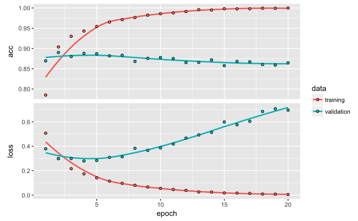
Word that the decision to match() returns a historical past object. The historical past object has a plot() technique that permits us to visualise the coaching and validation metrics by epoch:

The accuracy is plotted on the highest panel and the loss on the underside panel. Word that your individual outcomes could differ barely attributable to a special random initialization of your community.

As you may see, the coaching loss decreases with each epoch, and the coaching accuracy will increase with each epoch. That’s what you’d count on when operating a gradient-descent optimization – the amount you’re attempting to reduce needs to be much less with each iteration. However that isn’t the case for the validation loss and accuracy: they appear to peak on the fourth epoch. That is an instance of what we warned in opposition to earlier: a mannequin that performs higher on the coaching information isn’t essentially a mannequin that may do higher on information it has by no means seen earlier than. In exact phrases, what you’re seeing is overfitting: after the second epoch, you’re overoptimizing on the coaching information, and you find yourself studying representations which are particular to the coaching information and don’t generalize to information outdoors of the coaching set.

On this case, to stop overfitting, you could possibly cease coaching after three epochs. Usually, you should utilize a variety of methods to mitigate overfitting,which we’ll cowl in chapter 4.

Let’s practice a brand new community from scratch for 4 epochs after which consider it on the take a look at information.

mannequin <- keras_model_sequential() %>% 
  layer_dense(items = 16, activation = "relu", input_shape = c(10000)) %>% 
  layer_dense(items = 16, activation = "relu") %>% 
  layer_dense(items = 1, activation = "sigmoid")

mannequin %>% compile(
  optimizer = "rmsprop",
  loss = "binary_crossentropy",
  metrics = c("accuracy")
)

mannequin %>% match(x_train, y_train, epochs = 4, batch_size = 512)
outcomes <- mannequin %>% consider(x_test, y_test)

$loss
[1] 0.2900235

$acc
[1] 0.88512

This pretty naive strategy achieves an accuracy of 88%. With state-of-the-art approaches, it’s best to be capable to get near 95%.

Producing predictions

After having skilled a community, you’ll need to use it in a sensible setting. You may generate the chance of critiques being optimistic by utilizing the predict technique:

 [1,] 0.92306918
 [2,] 0.84061098
 [3,] 0.99952853
 [4,] 0.67913240
 [5,] 0.73874789
 [6,] 0.23108074
 [7,] 0.01230567
 [8,] 0.04898361
 [9,] 0.99017477
[10,] 0.72034937

As you may see, the community is assured for some samples (0.99 or extra, or 0.01 or much less) however much less assured for others (0.7, 0.2).

Additional experiments

The next experiments will assist persuade you that the structure decisions you’ve made are all pretty cheap, though there’s nonetheless room for enchancment.

• You used two hidden layers. Attempt utilizing one or three hidden layers, and see how doing so impacts validation and take a look at accuracy.
• Attempt utilizing layers with extra hidden items or fewer hidden items: 32 items, 64 items, and so forth.
• Attempt utilizing the mse loss perform as a substitute of binary_crossentropy.
• Attempt utilizing the tanh activation (an activation that was well-liked within the early days of neural networks) as a substitute of relu.

Wrapping up

Right here’s what it’s best to take away from this instance:

• You normally have to do fairly a little bit of preprocessing in your uncooked information so as to have the ability to feed it – as tensors – right into a neural community. Sequences of phrases could be encoded as binary vectors, however there are different encoding choices, too.
• Stacks of dense layers with relu activations can clear up a variety of issues (together with sentiment classification), and also you’ll probably use them ceaselessly.
• In a binary classification drawback (two output courses), your community ought to finish with a dense layer with one unit and a sigmoid activation: the output of your community needs to be a scalar between 0 and 1, encoding a chance.
• With such a scalar sigmoid output on a binary classification drawback, the loss perform it’s best to use is binary_crossentropy.
• The rmsprop optimizer is usually a adequate alternative, no matter your drawback. That’s one much less factor so that you can fear about.
• As they get higher on their coaching information, neural networks ultimately begin overfitting and find yourself acquiring more and more worse outcomes on information they’ve
  by no means seen earlier than. You should definitely at all times monitor efficiency on information that’s outdoors of the coaching set.