

That is the ultimate installment in a three-part collection on Twitter cluster analyses utilizing R and Gephi. Half one analyzed heated on-line dialogue about famed Argentine footballer Lionel Messi; half two deepened the evaluation to raised determine principal actors and perceive matter unfold.
Politics are polarizing. Once we discover attention-grabbing communities with drastically totally different opinions, Twitter messages generated from inside these camps are likely to densely cluster round two teams of customers, with a slight connection between them. The sort of grouping and relationship known as homophily: the tendency to work together with these much like us.
Within the earlier article on this collection, we centered on computational methods primarily based on Twitter knowledge units and have been in a position to generate informative visualizations by means of Gephi. Now we need to use cluster evaluation to grasp the conclusions we will draw from these methods and determine which social knowledge facets are most informative.
We are going to change the form of knowledge we analyze to spotlight this clustering, downloading United States’ political knowledge from Could 10, 2020, by means of Could 20, 2020. We’ll use the identical Twitter knowledge obtain course of we used within the first article on this collection, altering the obtain standards to the then-president’s title quite than “Messi.”
The next determine depicts the interplay graph of the political dialogue; as we did within the first article, we plotted this knowledge with Gephi utilizing the ForceAtlas2 structure and coloured by the communities as detected by Louvain.

Let’s dive deeper into the obtainable knowledge.
Who Are in These Clusters?
As we’ve mentioned all through this collection, we will characterize clusters by their authorities, however Twitter provides us much more knowledge that we will parse. For instance, the person’s description area, the place Twitter customers can present a short autobiography. Utilizing a phrase cloud, we will uncover how customers describe themselves. This code generates two phrase clouds primarily based on the phrase frequency discovered throughout the knowledge in every cluster’s descriptions and highlights how individuals’s self-descriptions are informative in an mixture approach:
# Load needed libraries
library(rtweet)
library(igraph)
library(tidyverse)
library(wordcloud)
library(tidyverse)
library(NLP)
library("tm")
library(RColorBrewer)


# First, determine the communities by means of Louvain
my.com.quick = cluster_louvain(as.undirected(simplify(internet)),decision=0.4)

# Subsequent, get the customers that conform to the 2 greatest clusters
largestCommunities <- order(sizes(my.com.quick), lowering=TRUE)[1:4]
community1 <- names(which(membership(my.com.quick) == largestCommunities[1]))
community2 <- names(which(membership(my.com.quick) == largestCommunities[2]))

# Now, break up the tweets’ knowledge frames by their communities
# (i.e., 'republicans' and 'democrats')

republicans = tweets.df[which(tweets.df$screen_name %in% community1),]
democrats = tweets.df[which(tweets.df$screen_name %in% community2),]

# Subsequent, on condition that we've one row per tweet and we need to analyze customers,
# let’s preserve just one row by person
accounts_r = republicans[!duplicated(republicans[,c('screen_name')]),]
accounts_d = democrats[!duplicated(democrats[,c('screen_name')]),]

# Lastly, plot the phrase clouds of the person’s descriptions by cluster

## Generate the Republican phrase cloud
## First, convert descriptions to tm corpus
corpus <- Corpus(VectorSource(distinctive(accounts_r$description)))

### Take away English cease phrases
corpus <- tm_map(corpus, removeWords, stopwords("en"))

### Take away numbers as a result of they aren't significant at this step
corpus <- tm_map(corpus, removeNumbers)

### Plot the phrase cloud displaying a most of 30 phrases
### Additionally, filter out phrases that seem solely as soon as
pal <- brewer.pal(8, "Dark2")
wordcloud(corpus, min.freq=2, max.phrases = 30, random.order = TRUE, col = pal)

## Generate the Democratic phrase cloud

corpus <- Corpus(VectorSource(distinctive(accounts_d$description)))
corpus <- tm_map(corpus, removeWords, stopwords("en"))
pal <- brewer.pal(8, "Dark2")
wordcloud(corpus, min.freq=2, max.phrases = 30, random.order = TRUE, col = pal)
Knowledge from earlier US elections reveals that voters are extremely segregated by geographical area. Let’s deepen our identification evaluation and deal with one other area: place_name, the sphere the place customers can present the place they reside. This R code generates phrase clouds primarily based on this area:
# Convert place names to tm corpus corpus <- Corpus(VectorSource(accounts_d[!is.na(accounts_d$place_name),]$place_name))

# Take away English cease phrases
corpus <- tm_map(corpus, removeWords, stopwords("en"))

# Take away numbers
corpus <- tm_map(corpus, removeNumbers)

# Plot
pal <- brewer.pal(8, "Dark2")
wordcloud(corpus, min.freq=2, max.phrases = 30, random.order = TRUE, col = pal)

## Do the identical for accounts_r
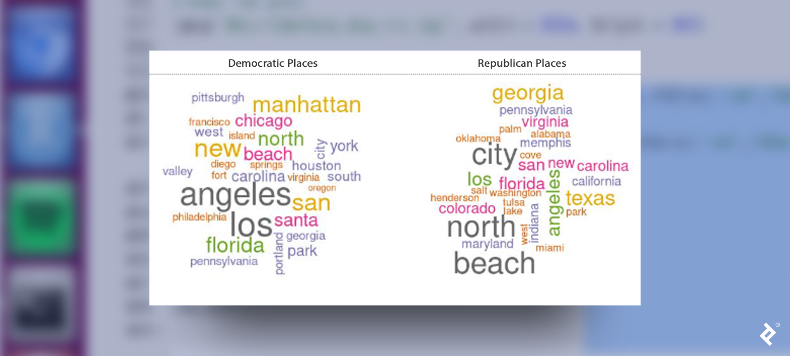
The names of some locations might seem in each phrase clouds as a result of voters in each events reside in most places. However some states, like Texas, Colorado, Oklahoma, and Indiana, strongly signify the Republican celebration whereas some cities, like New York, San Francisco, and Philadelphia, strongly correlate with the Democratic celebration.
Behaviors
Let’s discover one other aspect of the information, specializing in person habits and inspecting the distribution of when accounts inside every cluster have been created. If there is no such thing as a correlation between the creation date and the cluster, we’ll see a uniform distribution of customers for every day.
Let’s plot a histogram of the distribution:
# First we have to format the account date area to be successfully learn as Date
## Notice that we're utilizing the accounts_r and accounts_d knowledge body, it's because we need to deal with distinctive customers and don’t distort the plot by the variety of tweets that every person has submitted

accounts_r$date_account <- as.Date(format(as.POSIXct(accounts_r$account_created_at,format="%Y-%m-%d %H:%M:%S"),format="%Y-%m-%d"))

# Now we plot the histogram
ggplot(accounts_r, aes(date_account)) + geom_histogram(stat="depend")+scale_x_date(date_breaks = "1 12 months", date_labels = "%b %Y")

## Do the identical for accounts_d

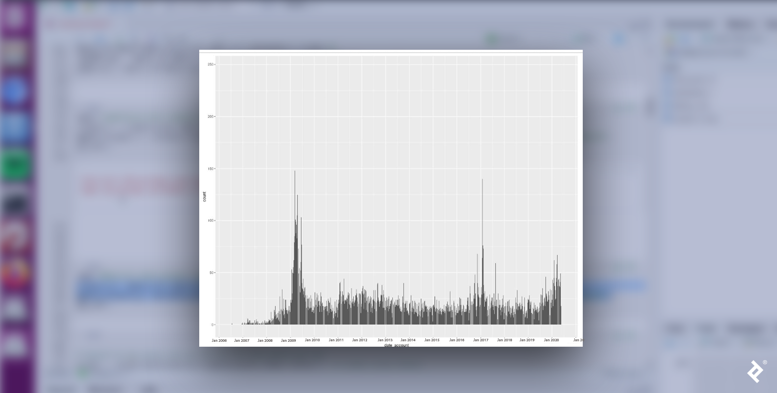
We see that Republican and Democratic customers are usually not distributed uniformly. In each circumstances, the variety of new person accounts peaked in January 2009 and January 2017, each months when inaugurations occurred following presidential elections within the Novembers of the earlier years. May or not it’s that the proximity to these occasions generates a rise in political dedication? That may make sense, on condition that we’re analyzing political tweets.
Additionally attention-grabbing to notice: The most important peak throughout the Republican knowledge happens after the center of 2019, reaching its highest worth in early 2020. May this transformation in habits be associated to digital habits introduced on by the pandemic?
The information for the Democrats additionally had a spike throughout this era however with a decrease worth. Possibly Republican supporters exhibited the next peak as a result of that they had stronger opinions about COVID lockdowns? We’d must rely extra on political information, theories, and findings to develop higher hypotheses, however regardless, there are attention-grabbing knowledge traits we will analyze from a political perspective.
One other approach to evaluate behaviors is to research how customers retweet and reply. When customers retweet, they unfold a message; nonetheless, once they reply, they contribute to a particular dialog or debate. Sometimes, the variety of replies correlates to a tweet’s diploma of divisiveness, unpopularity, or controversy; a person who favorites a tweet signifies settlement with the sentiment. Let’s study the ratio measure between the favorites and replies of a tweet.
Based mostly on homophily, we might count on customers to retweet customers from the identical group. We will confirm this with R:
# Get customers who've been retweeted by each side
rt_d = democrats[which(!is.na(democrats$retweet_screen_name)),]
rt_r = republicans[which(!is.na(republicans$retweet_screen_name)),]

# Retweets from democrats to republicans
rt_d_unique = rt_d[!duplicated(rt_d[,c('retweet_screen_name')]),]
rt_dem_to_rep = dim(rt_d_unique[which(rt_d_unique$retweet_screen_name %in% unique(republicans$screen_name)),])[1]/dim(rt_d_unique)[1]

# Retweets from democrats to democrats

rt_dem_to_dem = dim(rt_d_unique[which(rt_d_unique$retweet_screen_name %in% unique(democrats$screen_name)),])[1]/dim(rt_d_unique)[1]

# The rest
relaxation = 1 - rt_dem_to_dem - rt_dem_to_rep

# Create a dataframe to make the plot
knowledge <- knowledge.body(
  class=c( "Democrats","Republicans","Others"),
  depend=c(spherical(rt_dem_to_dem*100,1),spherical(rt_dem_to_rep*100,1),spherical(relaxation*100,1))
)

# Compute percentages
knowledge$fraction <- knowledge$depend / sum(knowledge$depend)

# Compute the cumulative percentages (prime of every rectangle)
knowledge$ymax <- cumsum(knowledge$fraction)

# Compute the underside of every rectangle
knowledge$ymin <- c(0, head(knowledge$ymax, n=-1))

# Compute label place
knowledge$labelPosition <- (knowledge$ymax + knowledge$ymin) / 2

# Compute a great label
knowledge$label <- paste0(knowledge$class, "n ", knowledge$depend)

# Make the plot

ggplot(knowledge, aes(ymax=ymax, ymin=ymin, xmax=4, xmin=3, fill=c('purple','blue','inexperienced'))) +
  geom_rect() +
  geom_text( x=1, aes(y=labelPosition, label=label, coloration=c('purple','blue','inexperienced')), dimension=6) + # x right here controls label place (internal / outer)

  coord_polar(theta="y") +
  xlim(c(-1, 4)) +
  theme_void() +
  theme(legend.place = "none")

# Do the identical for rt_r

As anticipated, Republicans are likely to retweet different Republicans and the identical is true for Democrats. Let’s see how celebration affiliation applies to tweet replies.

A really totally different sample emerges right here. Whereas customers are likely to reply extra usually to the tweets of people that share their celebration affiliation, they’re nonetheless more likely to retweet them. Additionally, it seems that individuals who don’t fall throughout the two principal clusters are likely to want to answer.
Through the use of the subject modeling method specified by half two of this collection, we will predict what sort of conversations customers will select to interact in with individuals of their identical cluster and with individuals of the alternative cluster.
The next desk particulars the 2 most essential subjects mentioned in every kind of interplay:
| Democrats to Democrats | Democrats to Republicans | Republicans to Democrats | Republicans to Republicans | ||||
| Matter 1 | Matter 2 | Matter 1 | Matter 2 | Matter 1 | Matter 2 | Matter 1 | Matter 2 |
| pretend | individuals | trump | people | information | biden | individuals | china |
| putin | covid | information | trump | pretend | obama | cash | information |
| election | virus | pretend | lifeless | cnn | obamagate | nation | individuals |
| cash | taking | lies | individuals | learn | joe | open | media |
| trump | lifeless | fox | deaths | fake_news | proof | again | pretend |
It seems that pretend information was a scorching matter when customers in our knowledge set replied. No matter a person’s celebration affiliation, once they replied to individuals from the opposite celebration, they talked about information channels sometimes favored by individuals of their explicit celebration. Secondly, when Democrats replied to different Democrats, they tended to speak about Putin, pretend elections, and COVID, whereas Republicans centered on stopping the lockdown and faux information from China.
Polarization Occurs
Polarization is a typical sample in social media, taking place everywhere in the world, not simply within the US. We’ve got seen how we will analyze group identification and habits in a polarized situation. With these instruments, anybody can reproduce cluster evaluation on an information set of their curiosity to see what patterns emerge. The patterns and outcomes from these analyses can each educate and assist generate additional exploration.
