
On this weblog put up, the MosaicML engineering group shares greatest practices for find out how to capitalize on fashionable open supply massive language fashions (LLMs) for manufacturing utilization. We additionally present pointers for deploying inference providers constructed round these fashions to assist customers of their collection of fashions and deployment {hardware}. We have now labored with a number of PyTorch-based backends in manufacturing; these pointers are drawn from our expertise with FasterTransformers, vLLM, NVIDIA’s soon-to-be-released TensorRT-LLM, and others.
Understanding LLM Textual content Era
Massive Language Fashions (LLMs) generate textual content in a two-step course of: “prefill”, the place the tokens within the enter immediate are processed in parallel, and “decoding”, the place textual content is generated one ‘token’ at a time in an autoregressive method. Every generated token is appended to the enter and fed again into the mannequin to generate the following token. Era stops when the LLM outputs a particular cease token or when a user-defined situation is met (e.g., some most variety of tokens has been generated). If you would like extra background on how LLMs use decoder blocks, try this weblog put up.
Tokens might be phrases or sub-words; the precise guidelines for splitting textual content into tokens differ from mannequin to mannequin. As an example, you possibly can evaluate how Llama fashions tokenize textual content to how OpenAI fashions tokenize textual content. Though LLM inference suppliers usually discuss efficiency in token-based metrics (e.g., tokens/second), these numbers should not at all times comparable throughout mannequin sorts given these variations. For a concrete instance, the group at Anyscale discovered that Llama 2 tokenization is nineteen% longer than ChatGPT tokenization (however nonetheless has a a lot decrease total value). And researchers at HuggingFace additionally discovered that Llama 2 required ~20% extra tokens to coach over the identical quantity of textual content as GPT-4.
Vital Metrics for LLM Serving
So, how precisely ought to we take into consideration inference pace?
Our group makes use of 4 key metrics for LLM serving:
- Time To First Token (TTFT): How shortly customers begin seeing the mannequin’s output after getting into their question. Low ready occasions for a response are important in real-time interactions, however much less essential in offline workloads. This metric is pushed by the point required to course of the immediate after which generate the primary output token.
- Time Per Output Token (TPOT): Time to generate an output token for every consumer that’s querying our system. This metric corresponds with how every consumer will understand the “pace” of the mannequin. For instance, a TPOT of 100 milliseconds/tok can be 10 tokens per second per consumer, or ~450 phrases per minute, which is quicker than a typical particular person can learn.
- Latency: The general time it takes for the mannequin to generate the complete response for a consumer. General response latency might be calculated utilizing the earlier two metrics: latency = (TTFT) + (TPOT) * (the variety of tokens to be generated).
- Throughput: The variety of output tokens per second an inference server can generate throughout all customers and requests.
Our aim? The quickest time to first token, the best throughput, and the quickest time per output token. In different phrases, we would like our fashions to generate textual content as quick as doable for as many customers as we will help.
Notably, there’s a tradeoff between throughput and time per output token: if we course of 16 consumer queries concurrently, we’ll have larger throughput in comparison with operating the queries sequentially, however we’ll take longer to generate output tokens for every consumer.
When you have total inference latency targets, listed below are some helpful heuristics for evaluating fashions:
- Output size dominates total response latency: For common latency, you possibly can often simply take your anticipated/max output token size and multiply it by an total common time per output token for the mannequin.
- Enter size isn’t vital for efficiency however essential for {hardware} necessities: The addition of 512 enter tokens will increase latency lower than the manufacturing of 8 extra output tokens within the MPT fashions. Nonetheless, the necessity to help lengthy inputs could make fashions tougher to serve. For instance, we suggest utilizing the A100-80GB (or newer) to serve MPT-7B with its most context size of 2048 tokens.
- General latency scales sub-linearly with mannequin dimension: On the identical {hardware}, bigger fashions are slower, however the pace ratio will not essentially match the parameter depend ratio. MPT-30B latency is ~2.5x that of MPT-7B latency. Llama2-70B latency is ~2x that of Llama2-13B latency.
We are sometimes requested by potential prospects to offer a mean inference latency. We suggest that earlier than you anchor your self to particular latency targets (“we want lower than 20 ms per token”), it is best to spend a while characterizing your anticipated enter and desired output lengths.
Challenges in LLM Inference
Optimizing LLM inference advantages from common methods equivalent to:
- Operator Fusion: Combining completely different adjoining operators collectively usually leads to higher latency.
- Quantization: Activations and weights are compressed to make use of a smaller variety of bits.
- Compression: Sparsity or Distillation.
- Parallelization: Tensor parallelism throughout a number of gadgets or pipeline parallelism for bigger fashions.
Past these strategies, there are lots of essential Transformer-specific optimizations. A primary instance of that is KV (key-value) caching. The Consideration mechanism in decoder-only Transformer-based fashions is computationally inefficient. Every token attends to all beforehand seen tokens, and thus recomputes most of the identical values as every new token is generated. For instance, whereas producing the Nth token, the (N-1)th token attends to (N-2)th, (N-3)th … 1st tokens. Equally, whereas producing (N+1)th token, consideration for the Nth token once more wants to take a look at the (N-1)th, (N-2)th, (N-3)th, … 1st tokens. KV caching, i.e., saving of intermediate keys/values for the eye layers, is used to protect these outcomes for later reuse, avoiding repeated computation.
Reminiscence Bandwidth is Key
Computations in LLMs are primarily dominated by matrix-matrix multiplication operations; these operations with small dimensions are sometimes memory-bandwidth-bound on most {hardware}. When producing tokens in an autoregressive method, one of many activation matrix dimensions (outlined by batch dimension and variety of tokens within the sequence) is small at small batch sizes. Due to this fact, the pace relies on how shortly we will load mannequin parameters from GPU reminiscence to native caches/registers, slightly than how shortly we will compute on loaded knowledge. Out there and achieved reminiscence bandwidth in inference {hardware} is a greater predictor of pace of token technology than their peak compute efficiency.
Inference {hardware} utilization is essential when it comes to serving prices. GPUs are costly and we want them to do as a lot work as doable. Shared inference providers promise to maintain prices low by combining workloads from many customers, filling in particular person gaps and batching collectively overlapping requests. For giant fashions like Llama2-70B, we solely obtain good value/efficiency at massive batch sizes. Having an inference serving system that may function at massive batch sizes is crucial for value effectivity. Nonetheless, a big batch means bigger KV cache dimension, and that in flip will increase the variety of GPUs required to serve the mannequin. There is a tug-of-war right here and shared service operators have to make some value trade-offs and implement methods optimizations.
Mannequin Bandwidth Utilization (MBU)
How optimized is an LLM inference server?
As briefly defined earlier, inference for LLMs at smaller batch sizes—particularly at decode time—is bottlenecked on how shortly we will load mannequin parameters from the machine reminiscence to the compute models. Reminiscence bandwidth dictates how shortly the info motion occurs. To measure the underlying {hardware}’s utilization, we introduce a brand new metric known as Mannequin Bandwidth Utilization (MBU). MBU is outlined as (achieved reminiscence bandwidth) / (peak reminiscence bandwidth) the place achieved reminiscence bandwidth is ((whole mannequin parameter dimension + KV cache dimension) / TPOT).
For instance, if a 7B parameter operating with 16-bit precision has TPOT equal to 14ms, then it is shifting 14GB of parameters in 14ms translating to 1TB/sec bandwidth utilization. If the height bandwidth of the machine is 2TB/sec, we’re operating at an MBU of fifty%. For simplicity, this instance ignores KV cache dimension, which is small for smaller batch sizes and shorter sequence lengths. MBU values near 100% suggest that the inference system is successfully using the obtainable reminiscence bandwidth. MBU can also be helpful to check completely different inference methods ({hardware} + software program) in a normalized method. MBU is complementary to the Mannequin Flops Utilization (MFU; launched in the PaLM paper) metric which is essential in compute-bound settings.
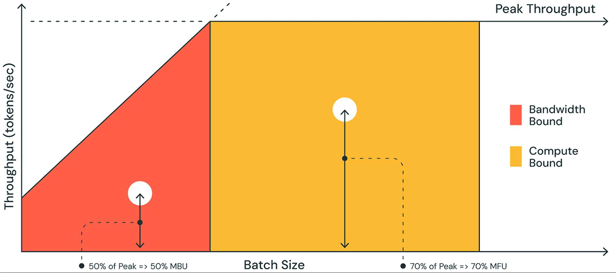
Determine 1 reveals a pictorial illustration of MBU in a plot much like a roofline plot. The strong sloped line of the orange-shaded area reveals the utmost doable throughput if reminiscence bandwidth is totally saturated at 100%. Nonetheless, in actuality for low batch sizes (white dot), the noticed efficiency is decrease than most – how a lot decrease is a measure of the MBU. For giant batch sizes (yellow area), the system is compute certain, and the achieved throughput as a fraction of the height doable throughput is measured because the Mannequin Flops Utilization (MFU).
MBU and MFU decide how far more room is obtainable to push the inference pace additional on a given {hardware} setup. Determine 2 reveals measured MBU for various levels of tensor parallelism with our TensorRT-LLM-based inference server. Peak reminiscence bandwidth utilization is attained when transferring massive contiguous reminiscence chunks. When smaller fashions like MPT-7B are distributed throughout a number of GPUs, we observe decrease MBU as we’re shifting smaller reminiscence chunks in every GPU.
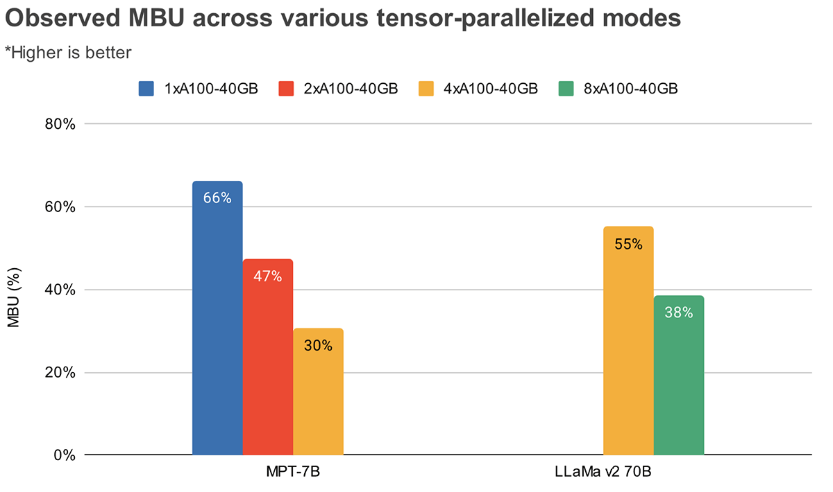
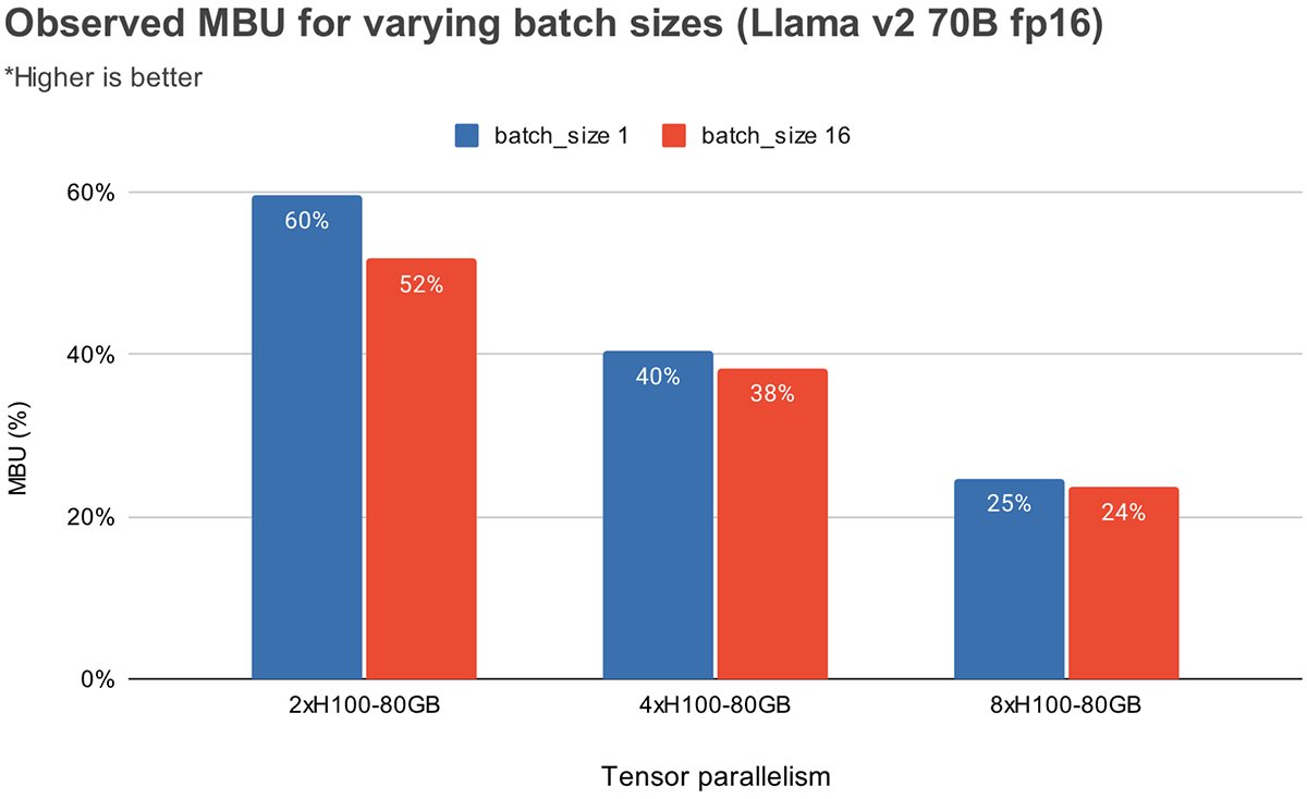
Determine 3 reveals empirically noticed MBU for various levels of tensor parallelism and batch sizes on the NVIDIA H100 GPUs. MBU decreases as batch dimension will increase. Nonetheless, as we scale GPUs, the relative lower in MBU is much less vital. It is usually worthy to notice that selecting {hardware} with higher reminiscence bandwidth can enhance efficiency with fewer GPUs. At batch dimension 1, we will obtain the next MBU of 60% on 2xH100-80GBs as in comparison with 55% on 4xA100-40GB GPUs (Determine 2).
Benchmarking Outcomes
Latency
We have now measured time to first token (TTFT) and time per output token (TPOT) throughout completely different levels of tensor parallelism for MPT-7B and Llama2-70B fashions. As enter prompts lengthen, time to generate the primary token begins to devour a considerable portion of whole latency. Tensor parallelizing throughout a number of GPUs helps scale back this latency.
In contrast to mannequin coaching, scaling to extra GPUs affords vital diminishing returns for inference latency. Eg. for Llama2-70B going from 4x to 8x GPUs solely decreases latency by 0.7x at small batch sizes. One purpose for that is that larger parallelism has decrease MBU (as mentioned earlier). Another excuse is that tensor parallelism introduces communication overhead throughout a GPU node.
| Time to first token (ms) | ||||
|---|---|---|---|---|
| Mannequin | 1xA100-40GB | 2xA100-40GB | 4xA100-40GB | 8xA100-40GB |
| MPT-7B | 46 (1x) | 34 (0.73x) | 26 (0.56x) | – |
| Llama2-70B | Would not match | 154 (1x) | 114 (0.74x) | |
Desk 1: Time to first token given enter requests are 512 tokens size with batch dimension of 1. Bigger fashions like Llama2 70B wants at the least 4xA100-40B GPUs to slot in reminiscence
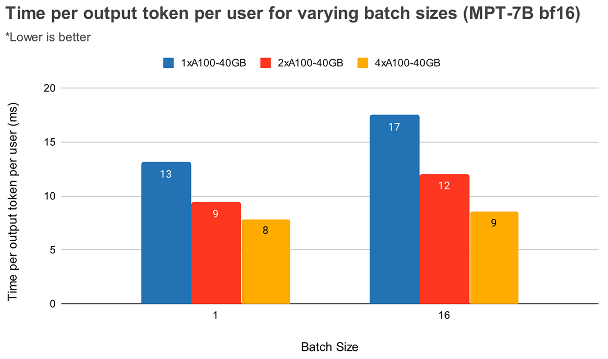
At bigger batch sizes, larger tensor parallelism results in a extra vital relative lower in token latency. Determine 4 reveals how time per output token varies for MPT-7B. At batch dimension 1, going from 2x to 4x solely reduces token latency by ~12%. At batch dimension 16, latency with 4x is 33% decrease than with 2x. This goes in keeping with our earlier statement that the relative lower in MBU is smaller at larger levels of tensor parallelism for batch dimension 16 as in comparison with batch dimension 1.
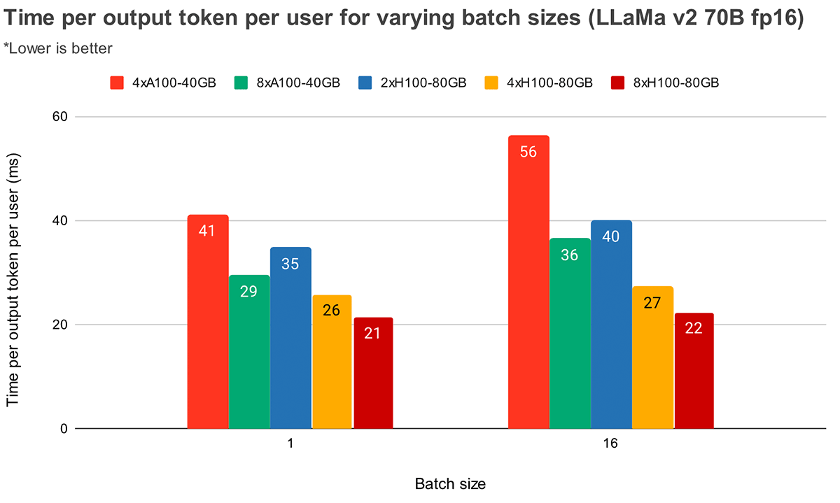
Determine 5 reveals related outcomes for Llama2-70B, besides the relative enchancment between 4x and 8x is much less pronounced. We additionally evaluate GPU scaling throughout two completely different {hardware}. As a result of H100-80GB has 2.15x GPU reminiscence bandwidth as in comparison with A100-40GB, we will see that latency is 36% decrease at batch dimension 1 and 52% decrease at batch dimension 16 for 4x methods.
Throughput
We are able to commerce off throughput and time per token by batching requests collectively. Grouping queries throughout GPU analysis will increase throughput in comparison with processing queries sequentially, however every question will take longer to finish (ignoring queueing results).
There are a number of frequent methods for batching inference requests:
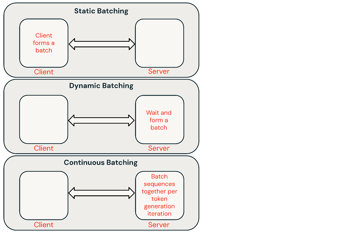
- Static batching: Shopper packs a number of prompts into requests and a response is returned in any case sequences within the batch have been accomplished. Our inference servers help this however don’t require it.
- Dynamic batching: Prompts are batched collectively on the fly contained in the server. Usually, this methodology performs worse than static batching however can get near optimum if responses are quick or of uniform size. Doesn’t work nicely when requests have completely different parameters.
- Steady batching: The thought of batching requests collectively as they arrive was launched in this glorious paper and is presently the SOTA methodology. As an alternative of ready for all sequences in a batch to complete, it teams sequences collectively on the iteration stage. It may well obtain 10x-20x higher throughput than dynamic batching.
Steady batching is often the most effective method for shared providers, however there are conditions the place the opposite two is likely to be higher. In low-QPS environments, dynamic batching can outperform steady batching. It’s generally simpler to implement low-level GPU optimizations in an easier batching framework. For offline batch inference workloads, static batching can keep away from vital overhead and obtain higher throughput.
Batch Measurement
How nicely batching works is extremely depending on the request stream. However we will get an higher certain on its efficiency by benchmarking static batching with uniform requests.
| Batch dimension | |||||||
|---|---|---|---|---|---|---|---|
| {Hardware} | 1 | 4 | 8 | 16 | 32 | 64 | 128 |
| 1 x A10 | 0.4 (1x) | 1.4 (3.5x) | 2.3 (6x) | 3.5 (9x) | OOM (Out of Reminiscence) error | ||
| 2 x A10 | 0.8 | 2.5 | 4.0 | 7.0 | 8.0 | ||
| 1 x A100 | 0.9 (1x) | 3.2 (3.5x) | 5.3 (6x) | 8.0 (9x) | 10.5 (12x) | 12.5 (14x) | |
| 2 x A100 | 1.3 | 3.0 | 5.5 | 9.5 | 14.5 | 17.0 | 22.0 |
| 4 x A100 | 1.7 | 6.2 | 11.5 | 18.0 | 25.0 | 33.0 | 36.5 |
Desk 2: Peak MPT-7B throughput (req/sec) with static batching and a FasterTransformers-based backend. Requests: 512 enter and 64 output tokens. For bigger inputs, the OOM boundary will likely be at smaller batch sizes.
Latency Commerce-Off
Request latency will increase with batch dimension. With one NVIDIA A100 GPU, for instance, if we maximize throughput with a batch dimension of 64, latency will increase by 4x whereas throughput will increase by 14x. Shared inference providers sometimes choose a balanced batch dimension. Customers internet hosting their very own fashions ought to determine the suitable latency/throughput trade-off for his or her purposes. In some purposes, like chatbots, low latency for quick responses is the highest precedence. In different purposes, like batched processing of unstructured PDFs, we would wish to sacrifice the latency to course of a person doc to course of all of them quick in parallel.
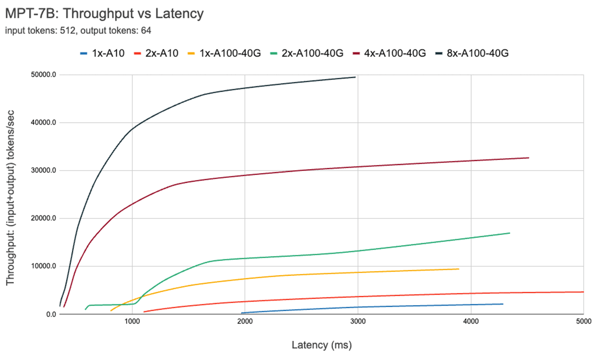
Determine 7 reveals the throughput vs latency curve for the 7B mannequin. Every line on this curve is obtained by growing the batch dimension from 1 to 256. That is helpful in figuring out how massive we will make the batch dimension, topic to completely different latency constraints. Recalling our roofline plot above, we discover that these measurements are per what we’d anticipate. After a sure batch dimension, i.e., after we cross to the compute certain regime, each doubling of batch dimension simply will increase the latency with out growing throughput.
When utilizing parallelism, it is essential to know low-level {hardware} particulars. As an example, not all 8xA100 cases are the identical throughout completely different clouds. Some servers have excessive bandwidth connections between all GPUs, others pair GPUs and have decrease bandwidth connections between pairs. This might introduce bottlenecks, inflicting real-world efficiency to deviate considerably from the curves above.
Optimization Case Examine: Quantization
Quantization is a standard approach used to scale back the {hardware} necessities for LLM inference. Decreasing the precision of mannequin weights and activations throughout inference can dramatically scale back {hardware} necessities. As an example, switching from 16-bit weights to 8-bit weights can halve the variety of required GPUs in reminiscence constrained environments (eg. Llama2-70B on A100s). Dropping right down to 4-bit weights makes it doable to run inference on client {hardware} (eg. Llama2-70B on Macbooks).
In our expertise, quantization must be carried out with warning. Naive quantization methods can result in a considerable degradation in mannequin high quality. The affect of quantization additionally varies throughout mannequin architectures (eg. MPT vs Llama) and sizes. We’ll discover this in additional element in a future weblog put up.
When experimenting with methods like quantization, we suggest utilizing an LLM high quality benchmark just like the Mosaic Eval Gauntlet to guage the standard of the inference system, not simply the standard of the mannequin in isolation. Moreover, it is essential to discover deeper methods optimizations. Specifically, quantization could make KV caches far more environment friendly.
As talked about beforehand, in autoregressive token technology, previous Key/Values (KV) from the eye layers are cached as an alternative of recomputing them at each step. The scale of the KV cache varies based mostly on the variety of sequences processed at a time and the size of those sequences. Furthermore, throughout every iteration of the following token technology, new KV objects are added to the prevailing cache making it larger as new tokens are generated. Due to this fact, efficient KV cache reminiscence administration when including these new values is crucial for good inference efficiency. Llama2 fashions use a variant of consideration known as Grouped Question Consideration (GQA). Please word that when the variety of KV heads is 1, GQA is identical as Multi-Question-Consideration (MQA). GQA helps with maintaining the KV cache dimension down by sharing Keys/Values. The method to calculate KV cache dimension isbatch_size * seqlen * (d_model/n_heads) * n_layers * 2 (Ok and V) * 2 (bytes per Float16) * n_kv_heads
Desk 3 reveals GQA KV cache dimension calculated at completely different batch sizes at a sequence size of 1024 tokens. The parameter dimension for Llama2 fashions, compared, is 140 GB (Float16) for the 70B mannequin. Quantization of KV cache is one other approach (along with GQA/MQA) to scale back the dimensions of KV cache, and we’re actively evaluating its affect on the technology high quality.
| Batch Measurement | GQA KV cache reminiscence (FP16) | GQA KV cache reminiscence (Int8) |
|---|---|---|
| 1 | .312 GiB | .156 GiB |
| 16 | 5 GiB | 2.5 GiB |
| 32 | 10 GiB | 5 GiB |
| 64 | 20 GiB | 10 GiB |
Desk 3: KV cache dimension for Llama-2-70B at a sequence size of 1024
As talked about beforehand, token technology with LLMs at low batch sizes is a GPU reminiscence bandwidth-bound downside, i.e. the pace of technology is dependent upon how shortly mannequin parameters might be moved from the GPU reminiscence to on-chip caches. Changing mannequin weights from FP16 (2 bytes) to INT8 (1 byte) or INT4 (0.5 byte) requires shifting much less knowledge and thus hurries up token technology. Nonetheless, quantization could negatively affect the mannequin technology high quality. We’re presently evaluating the affect on mannequin high quality utilizing Mannequin Gauntlet and plan to publish a followup weblog put up on it quickly.
Conclusions and Key Outcomes
Every of the elements we have outlined above influences the best way we construct and deploy fashions. We use these outcomes to make data-driven selections that consider the {hardware} kind, the software program stack, the mannequin structure, and typical utilization patterns. Listed here are some suggestions drawn from our expertise.
Establish your optimization goal: Do you care about interactive efficiency? Maximizing throughput? Minimizing value? There are predictable trade-offs right here.
Take note of the parts of latency: For interactive purposes time-to-first-token drives how responsive your service will really feel and time-per-output-token determines how briskly it’ll really feel.
Reminiscence bandwidth is essential: Producing the primary token is often compute-bound, whereas subsequent decoding is memory-bound operation. As a result of LLM inference usually operates in memory-bound settings, MBU is a helpful metric to optimize for and can be utilized to check the effectivity of inference methods.
Batching is crucial: Processing a number of requests concurrently is crucial for reaching excessive throughput and for successfully using costly GPUs. For shared on-line providers steady batching is indispensable, whereas offline batch inference workloads can obtain excessive throughput with easier batching methods.
In depth optimizations: Normal inference optimization methods are essential (eg. operator fusion, weight quantization) for LLMs nevertheless it’s essential to discover deeper methods optimizations, particularly these which enhance reminiscence utilization. One instance is KV cache quantization.
{Hardware} configurations: The mannequin kind and anticipated workload must be used to determine deployment {hardware}. As an example, when scaling to a number of GPUs MBU falls far more quickly for smaller fashions, equivalent to MPT-7B, than it does for bigger fashions, equivalent to Llama2-70B. Efficiency additionally tends to scale sub-linearly with larger levels of tensor parallelism. That mentioned, a excessive diploma of tensor parallelism would possibly nonetheless make sense for smaller fashions if visitors is excessive or if customers are prepared to pay a premium for additional low latency.
Knowledge Pushed Selections: Understanding the speculation is essential, however we suggest at all times measuring end-to-end server efficiency. There are numerous causes an inference deployment can carry out worse than anticipated. MBU may very well be unexpectedly low due to software program inefficiencies. Or variations in {hardware} between cloud suppliers may result in surprises (we have now noticed a 2x latency distinction between 8xA100 servers from two cloud suppliers).
To get began with LLM inference, check out Databricks Mannequin Serving. Take a look at the documentation to study extra.
