
We’re excited to announce that the keras bundle is now accessible on CRAN. The bundle gives an R interface to Keras, a high-level neural networks API developed with a give attention to enabling quick experimentation. Keras has the next key options:
-
Permits the identical code to run on CPU or on GPU, seamlessly.
-
Person-friendly API which makes it simple to rapidly prototype deep studying fashions.
-
Constructed-in help for convolutional networks (for laptop imaginative and prescient), recurrent networks (for sequence processing), and any mixture of each.
-
Helps arbitrary community architectures: multi-input or multi-output fashions, layer sharing, mannequin sharing, and so forth. Which means that Keras is suitable for constructing basically any deep studying mannequin, from a reminiscence community to a neural Turing machine.
-
Is able to operating on high of a number of back-ends together with TensorFlow, CNTK, or Theano.
If you’re already aware of Keras and need to bounce proper in, take a look at https://tensorflow.rstudio.com/keras which has every thing you should get began together with over 20 full examples to study from.
To study a bit extra about Keras and why we’re so excited to announce the Keras interface for R, learn on!
Keras and Deep Studying
Curiosity in deep studying has been accelerating quickly over the previous few years, and several other deep studying frameworks have emerged over the identical timeframe. Of all of the accessible frameworks, Keras has stood out for its productiveness, flexibility and user-friendly API. On the similar time, TensorFlow has emerged as a next-generation machine studying platform that’s each extraordinarily versatile and well-suited to manufacturing deployment.
Not surprisingly, Keras and TensorFlow have of late been pulling away from different deep studying frameworks:
Google net search curiosity round deep studying frameworks over time. For those who bear in mind This autumn 2015 and Q1-2 2016 as complicated, you were not alone. pic.twitter.com/1f1VQVGr8n
— François Chollet (@fchollet) June 3, 2017
The excellent news about Keras and TensorFlow is that you simply don’t want to decide on between them! The default backend for Keras is TensorFlow and Keras might be built-in seamlessly with TensorFlow workflows. There may be additionally a pure-TensorFlow implementation of Keras with deeper integration on the roadmap for later this 12 months.
Keras and TensorFlow are the cutting-edge in deep studying instruments and with the keras bundle now you can entry each with a fluent R interface.
Getting Began
Set up
To start, set up the keras R bundle from CRAN as follows:
The Keras R interface makes use of the TensorFlow backend engine by default. To put in each the core Keras library in addition to the TensorFlow backend use the install_keras() operate:
It will give you default CPU-based installations of Keras and TensorFlow. If you need a extra personalized set up, e.g. if you wish to make the most of NVIDIA GPUs, see the documentation for install_keras().
MNIST Instance
We will study the fundamentals of Keras by strolling by means of a easy instance: recognizing handwritten digits from the MNIST dataset. MNIST consists of 28 x 28 grayscale photographs of handwritten digits like these:

The dataset additionally consists of labels for every picture, telling us which digit it’s. For instance, the labels for the above photographs are 5, 0, 4, and 1.
Getting ready the Information
The MNIST dataset is included with Keras and might be accessed utilizing the dataset_mnist() operate. Right here we load the dataset then create variables for our check and coaching knowledge:
The x knowledge is a 3D array (photographs,width,peak) of grayscale values. To arrange the information for coaching we convert the 3D arrays into matrices by reshaping width and peak right into a single dimension (28×28 photographs are flattened into size 784 vectors). Then, we convert the grayscale values from integers ranging between 0 to 255 into floating level values ranging between 0 and 1:
The y knowledge is an integer vector with values starting from 0 to 9. To arrange this knowledge for coaching we one-hot encode the vectors into binary class matrices utilizing the Keras to_categorical() operate:
y_train <- to_categorical(y_train, 10)
y_test <- to_categorical(y_test, 10)
Defining the Mannequin
The core knowledge construction of Keras is a mannequin, a approach to manage layers. The best kind of mannequin is the sequential mannequin, a linear stack of layers.
We start by making a sequential mannequin after which including layers utilizing the pipe (%>%) operator:
mannequin <- keras_model_sequential()
mannequin %>%
  layer_dense(models = 256, activation = "relu", input_shape = c(784)) %>%
  layer_dropout(price = 0.4) %>%
  layer_dense(models = 128, activation = "relu") %>%
  layer_dropout(price = 0.3) %>%
  layer_dense(models = 10, activation = "softmax")
The input_shape argument to the primary layer specifies the form of the enter knowledge (a size 784 numeric vector representing a grayscale picture). The ultimate layer outputs a size 10 numeric vector (possibilities for every digit) utilizing a softmax activation operate.
Use the abstract() operate to print the small print of the mannequin:
Mannequin
________________________________________________________________________________
Layer (kind)                        Output Form                    Param #
================================================================================
dense_1 (Dense)                     (None, 256)                     200960
________________________________________________________________________________
dropout_1 (Dropout)                 (None, 256)                     0
________________________________________________________________________________
dense_2 (Dense)                     (None, 128)                     32896
________________________________________________________________________________
dropout_2 (Dropout)                 (None, 128)                     0
________________________________________________________________________________
dense_3 (Dense)                     (None, 10)                      1290
================================================================================
Whole params: 235,146
Trainable params: 235,146
Non-trainable params: 0
________________________________________________________________________________
Subsequent, compile the mannequin with acceptable loss operate, optimizer, and metrics:
mannequin %>% compile(
  loss = "categorical_crossentropy",
  optimizer = optimizer_rmsprop(),
  metrics = c("accuracy")
)
Coaching and Analysis
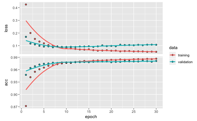
Use the match() operate to coach the mannequin for 30 epochs utilizing batches of 128 photographs:
historical past <- mannequin %>% match(
  x_train, y_train,
  epochs = 30, batch_size = 128,
  validation_split = 0.2
)
The historical past object returned by match() consists of loss and accuracy metrics which we are able to plot:

Consider the mannequin’s efficiency on the check knowledge:
mannequin %>% consider(x_test, y_test,verbose = 0)$loss
[1] 0.1149
$acc
[1] 0.9807Generate predictions on new knowledge:
mannequin %>% predict_classes(x_test) [1] 7 2 1 0 4 1 4 9 5 9 0 6 9 0 1 5 9 7 3 4 9 6 6 5 4 0 7 4 0 1 3 1 3 4 7 2 7 1 2
[40] 1 1 7 4 2 3 5 1 2 4 4 6 3 5 5 6 0 4 1 9 5 7 8 9 3 7 4 6 4 3 0 7 0 2 9 1 7 3 2
[79] 9 7 7 6 2 7 8 4 7 3 6 1 3 6 9 3 1 4 1 7 6 9
[ reached getOption("max.print") -- omitted 9900 entries ]Keras gives a vocabulary for constructing deep studying fashions that’s easy, elegant, and intuitive. Constructing a query answering system, a picture classification mannequin, a neural Turing machine, or every other mannequin is simply as easy.
The Information to the Sequential Mannequin article describes the fundamentals of Keras sequential fashions in additional depth.
Examples
Over 20 full examples can be found (particular because of [@dfalbel](https://github.com/dfalbel) for his work on these!). The examples cowl picture classification, textual content era with stacked LSTMs, question-answering with reminiscence networks, switch studying, variational encoding, and extra.
| addition_rnn | Implementation of sequence to sequence studying for performing addition of two numbers (as strings). |
| babi_memnn | Trains a reminiscence community on the bAbI dataset for studying comprehension. |
| babi_rnn | Trains a two-branch recurrent community on the bAbI dataset for studying comprehension. |
| cifar10_cnn | Trains a easy deep CNN on the CIFAR10 small photographs dataset. |
| conv_lstm | Demonstrates the usage of a convolutional LSTM community. |
| deep_dream | Deep Desires in Keras. |
| imdb_bidirectional_lstm | Trains a Bidirectional LSTM on the IMDB sentiment classification activity. |
| imdb_cnn | Demonstrates the usage of Convolution1D for textual content classification. |
| imdb_cnn_lstm | Trains a convolutional stack adopted by a recurrent stack community on the IMDB sentiment classification activity. |
| imdb_fasttext | Trains a FastText mannequin on the IMDB sentiment classification activity. |
| imdb_lstm | Trains a LSTM on the IMDB sentiment classification activity. |
| lstm_text_generation | Generates textual content from Nietzsche’s writings. |
| mnist_acgan | Implementation of AC-GAN (Auxiliary Classifier GAN ) on the MNIST dataset |
| mnist_antirectifier | Demonstrates write customized layers for Keras |
| mnist_cnn | Trains a easy convnet on the MNIST dataset. |
| mnist_irnn | Copy of the IRNN experiment with pixel-by-pixel sequential MNIST in “A Easy Approach to Initialize Recurrent Networks of Rectified Linear Models” by Le et al. |
| mnist_mlp | Trains a easy deep multi-layer perceptron on the MNIST dataset. |
| mnist_hierarchical_rnn | Trains a Hierarchical RNN (HRNN) to categorise MNIST digits. |
| mnist_transfer_cnn | Switch studying toy instance. |
| neural_style_transfer | Neural fashion switch (producing a picture with the identical “content material” as a base picture, however with the “fashion” of a unique image). |
| reuters_mlp | Trains and evaluates a easy MLP on the Reuters newswire matter classification activity. |
| stateful_lstm | Demonstrates use stateful RNNs to mannequin lengthy sequences effectively. |
| variational_autoencoder | Demonstrates construct a variational autoencoder. |
| variational_autoencoder_deconv | Demonstrates construct a variational autoencoder with Keras utilizing deconvolution layers. |
Studying Extra
After you’ve turn out to be aware of the fundamentals, these articles are an excellent subsequent step:
-
Information to the Sequential Mannequin. The sequential mannequin is a linear stack of layers and is the API most customers ought to begin with.
-
Information to the Purposeful API. The Keras practical API is the way in which to go for outlining advanced fashions, similar to multi-output fashions, directed acyclic graphs, or fashions with shared layers.
-
Coaching Visualization. There are all kinds of instruments accessible for visualizing coaching. These embody plotting of coaching metrics, actual time show of metrics throughout the RStudio IDE, and integration with the TensorBoard visualization device included with TensorFlow.
-
Utilizing Pre-Skilled Fashions. Keras consists of numerous deep studying fashions (Xception, VGG16, VGG19, ResNet50, InceptionVV3, and MobileNet) which can be made accessible alongside pre-trained weights. These fashions can be utilized for prediction, function extraction, and fine-tuning.
-
Incessantly Requested Questions. Covers many extra subjects together with streaming coaching knowledge, saving fashions, coaching on GPUs, and extra.
Keras gives a productive, extremely versatile framework for creating deep studying fashions. We will’t wait to see what the R neighborhood will do with these instruments!
